The Effects of Rising Student Costs in Higher Education

In Virginia and elsewhere, higher education faces an unstable future. Demographic, economic and technological changes are driving transformation in all that we do. Higher education – access to it, knowledge created and disseminated through it, and outcomes produced by it – will be the key to innovation and prosperity. At the same time, public higher education faces an unprecedentedly challenging landscape as it seeks to fulfill its public purposes and responsibilities. Its transformative potential for our nation is at risk.

The risk is most evident in the ever-increasing tuition our colleges and universities charge. Regardless of the reasons, higher prices mean fewer families can gain the education and training they need to grow and prosper in their communities. Traditionally-underserved students, as well as families from deeper into the middle class, find it difficult to afford a college education.  State and federal financial aid is not meeting the growing need, and more students face higher debt levels. While enrollment in higher education is leveling off, if not declining, demand for completers of postsecondary credentials has never been higher. We ignore these divergences at our peril.

Acutely aware of these challenges and trends, the State Council of Higher Education for Virginia spent much of 2014 developing the next statewide strategic plan for Virginia higher education. Our plan’s goals are as unsurprising as they are daunting – affordable access, student success, innovative change and improvement, and economic and cultural prosperity. Here, too, higher education’s purposes and responsibilities are central, and how to achieve their fulfillment, regardless of funding, remains the issue.

Ithaka S+R entered this swirling environment with a set of promising questions: What has been the impact of tuition and fee increases on enrollment patterns, student access and graduation? What strategies might the Commonwealth take to ensure affordable access to high-quality institutions? The findings corroborate and expand on what SCHEV has observed in its studies on the erosion of public funding – namely, reduced public funding diminishes institutional capacity, and higher prices threaten broad access. On many levels, we do not deserve the breadth and quality of our colleges and universities.

Dick Spies and his colleagues have done a tremendous job of consolidating data from a variety of sources (including SCHEV’s notable research site, http://research.schev.edu/ ), analyzing these data in creative ways, and articulating on-target explanations and conclusions. It has been no small task, and the report’s potential to inform conversations on the purposes and responsibilities of public higher education – and more importantly, public higher education’s ability to fulfill them – is equally large.

The team at Ithaka S+R was thoughtful, flexible and gracious throughout this effort. Virginia and its system of public higher education could not have asked for a more committed, skillful partner in this analysis. The Commonwealth will benefit from this work, and I am certain other states will as well.

Peter Blake, SCHEV Director

Acknowledgements

This study was undertaken by Ithaka S+R in partnership with the State Council of Higher Education for Virginia (SCHEV) and with the support of The Andrew W. Mellon Foundation. It arises out of a concern that public higher education, especially since the Great Recession that began in 2007-08, has not been able to produce a sufficient number of college graduates to satisfy regional and national needs for a better educated workforce, nor to function effectively as an accessible and affordable vehicle for less advantaged citizens to achieve economic and social mobility. In our view, Virginia represents an ideal setting to determine the extent to which this concern is supported by the evidence and, if so, what options are available for both the public institutions and the states that support them to do a better job of meeting these public responsibilities.

We are grateful to the Board and staff of SCHEV for their commitment to this project and for their willingness to assemble the very large database that we used to analyze these questions.^[1] We are also grateful to The Andrew W. Mellon Foundation for its support for this project. Finally, we acknowledge with appreciation the many contributions of our colleagues at Ithaka S+R.^[2]

Section 1: Purpose and Overview

Our Study

This study documents funding shifts for public higher education following the Great Recession and analyzes how different groups of institutions in Virginia have responded to those shifts. Our hypothesis is that the shift from a funding model largely supported by state appropriations to one primarily dependent on tuition revenue has made it more difficult for young people to pursue, and ultimately secure, a college degree at public institutions in Virginia. Moreover, to the extent that need-based financial aid programs in those institutions have not kept pace with rising student charges, we posit that students who come from economically disadvantaged backgrounds have been disproportionately affected. We chose to study Virginia because of the interest of the leadership of the State Council of Higher Education for Virginia (SCHEV) in better understanding these issues, the very rich database that SCHEV has built over time, and the similarities that its challenges hold to those of other states. We employ a micro-level dataset from SCHEV that contains observations covering more than 1.4 million students who enrolled in a public institution in Virginia between the 1997-98 and 2012-13 academic years.^[3] The very high degree of completeness and accuracy of the data used in this study – which encompass the entirety (and not just a sample) of the public college-enrolling population in Virginia – sets it apart from previous studies that have analyzed these issues, and provides a powerful empirical foundation upon which to estimate the relationships and draw the conclusions that we describe in this report.

As this report will detail, we found significant evidence that public higher education in Virginia is falling well short in its efforts to meet broader national goals of increasing overall educational attainment and narrowing the gaps that exist in educational levels between students from different socioeconomic backgrounds. Declining state appropriations and increasing reliance on tuition revenue have substantially increased the cost of public higher education to Virginia students, and the trend has accelerated since the Great Recession that began in 2007. Rising costs have deterred students from remaining in college and completing their degrees, and the lowest-income students have been hit the hardest. These results are particularly discouraging given that public higher education as a whole in Virginia – as in most states – was already falling well short of achieving these goals even before the latest declines in state support and increases in tuition came into effect. This study measures the degree to which these trends have worsened since the Great Recession and raises the alarm about what the future will be like if nothing is done to turn the present situation around.

Public Higher Education: Mission and Challenges

The central mission of public higher education in this country is to educate and prepare young adults to assume productive roles in a modern workforce, contribute to our national and regional economic competitiveness, strengthen our communities and nation as educated and caring citizens, and live enriching lives. As part of the special American dream of “equal opportunity for all,” public higher education also plays a critical role in seeking to eliminate, or at least narrow, gaps in opportunity between young people born into different socioeconomic circumstances. As far back as the Morrill Act of 1862 (which created our system of state-supported land grant universities), these goals have been the hallmark of American public higher education.^[4]

In recent years, the first goal of increasing the number of college graduates in the U.S. has received wide attention from various policymakers and stakeholders. Most notably, in 2009, President Obama proposed that by 2020 America would once again have the highest proportion of college graduates in the world.^[5] To reach this goal, the U.S. would need more than 65% of individuals between the ages 25 and 34 to possess a college degree.^[6] Various private foundations (including Gates and Lumina) have established similar targets in recent years to challenge colleges and universities to respond accordingly.^[7] While the specific goals and timetables vary, the need for more better-educated young people to enter and build our workforce – and, by extension, our citizenry – has never been clearer.

The second goal of reducing the opportunity gap between students from different socioeconomic backgrounds is also critical, both in itself and as a means to increase overall educational attainment in our society. Starting with the GI Bill of the post-World War II era and the original Higher Education Act of 1965, the goal of equalizing opportunity has received broad public endorsement at the national, state, and local levels. Public colleges and universities are critically important in that effort, as they educate a large majority of low- and middle-income students. Furthermore, President Obama’s recent call to make community college tuition-free is aimed directly at shrinking the opportunity gap by removing some of the cost barriers to higher education access and degree attainment.^[8]

National Context

Notwithstanding this high-level attention, progress on both of these goals remains discouragingly slow. Nationally, only 42% of 24-35 year olds had a post-secondary degree as of 2012.^[9] While the enrollment rate of 18-24 year olds in postsecondary education modestly improved from 39% to 42% between 2007 and 2011, this rate dropped to 41% in 2012.^[10] More importantly, current enrollment rates are much too low to produce a significant change in the overall number of degree holders, and too many students who do enroll at a post-secondary institution leave without a degree.^[11] Finally, a student from an upper-income family where at least one parent has a college degree is almost eight times more likely to get a college degree than a student from a low-income family where neither of the parents has a college degree – dramatic proof of a very large gap between the educational opportunities available for different socioeconomic groups.^[12]

Affordability and access to higher education are challenges for most public institutions, and states and institutions wrestle annually with the specific challenges associated with setting tuition and fees and providing adequate funding for need-based financial aid programs. In 2012, for the first time since the turn of the century, tuition as a share of total revenue surpassed the share associated with state funding for public institutions nationwide.^[13] At the same time, states and institutions are trying to do more to improve student outcomes and reduce the gaps between less advantaged students and their more well-to-do counterparts.

Unfortunately, despite significant efforts on the part of many state and institutional leaders, not enough progress has been made to meet the goals of increasing the number of college graduates and decreasing the opportunity gap between students from different socioeconomic backgrounds. Significant reductions in state appropriations for higher education have made it difficult to support even current enrollment levels, with 49 states spending less per undergraduate in 2011-2012 than before the Great Recession, and 28 states actually decreasing per-student funding by more than 25 percent since 2008.^[14] In particular, the Great Recession that officially began in 2007 weakened not only state budgets but also the priority given to higher education within those budgets.^[15] Colleges and universities historically dependent on public support began increasingly to rely on tuition and other student charges for the resources needed to support their programs, with tuition charges at public four-year institutions increasing by a national average of 20% between 2008 and 2012.^[16] Concurrently, stagnating family incomes have resulted in tuition as a fraction of family income growing by 3.5% from 2008 to 2012.^[17]

Similar financial patterns are evident in Virginia, which currently provides only about half as much support per student at public institutions as it did in 2001.^[18] Virginia ranked 35^th nationwide in state funding per FTE (full-time equivalent) as of 2011-2012, and it has seen average tuition as a share of family income at public four-year institutions rise by 3.9% (slightly above the national average) from 2008 to 2012.^[19] Thus, in terms of these financial challenges, Virginia seems to be a microcosm of the public higher education scene in the country. Given that Virginia is also an economically and demographically diverse state with characteristics similar to the national average, we believe that the conclusions drawn from our analysis of financial trends and student outcomes in Virginia apply broadly to many other states and public institutions.^[20]

Summary of the Results

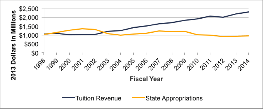
Over the past decade and a half, there has been a dramatic shift in Virginia higher education financing away from state appropriations and toward tuition.

Over the past decade and a half, there has been a dramatic shift in Virginia higher education financing away from state appropriations and toward tuition. Inflation-adjusted state appropriations in Virginia declined by 30% between fiscal years 2001 and 2014 (Figure 1.1). As a result, nearly every public institution has had to become significantly more dependent on tuition revenue in order to pay for the resources they need, ranging from faculty salaries to financial aid (see Section 2).

While decreases in state funding are not unprecedented, there are several factors that make the significant declines since the beginning of the Great Recession in 2007 particularly concerning; these include the severity of the most recent recession, the proximity and compounding nature of the last two recessions (in 2001 and 2007), and the large increases in enrollment that have placed additional pressures on state resources. Based on the state’s recent budgets, it does not appear likely that this situation will be significantly repaired or reversed in the foreseeable future.

Figure 1.1. Total Revenue from Tuition and State Appropriations

Different institutions within Virginia have taken somewhat different approaches in responding to the challenges represented by the decline in public funding, but tuition levels have nevertheless gone up significantly for all institutions, while financial aid programs have generally not been able to keep pace. The key measure of student costs used in this study is inflation-adjusted net costs, defined as the difference between a student’s estimated cost of attendance and the total amount of gift aid received for an academic year. Based on our analysis of data for 1,450,321 students who enrolled in a Virginia public institution between the 1997-1998 and 2012-2013 academic years, net costs at four-year public institutions have increased at rates well above inflation for in-state, full-time, first-time freshmen from most socioeconomic groups since 1997 (see Section 3).^[21] Furthermore, these increases have accelerated since the recession began in 2007, as many institutions expanded student charges and/or cut back on need-based financial aid.

Between 2007 and 2012, net costs grew 3.5% per year above inflation for the lowest income quintile, compared to lower rates for the other income groups.

It is especially worrying that, since 2007, net costs have grown fastest for the lowest income students (Table 1.1). Between 2007 and 2012, net costs grew 3.5% per year above inflation for the lowest income quintile, compared to lower rates for the other income groups.^[22] This represents a significant change from the pattern prior to 2007, when net costs grew fastest for the highest-income students and stayed almost flat for the poorest students.

Table 1.1. Average Annual Growth Rates in Net Costs at Four-Year Institutions by Income Quintile

	1st Quintile	3rd Quintile	5th Quintile
1997-2007	-0.2%	1.9%	1.8%
2007-2012	3.5%	3.2%	2.6%
Total (1997-2012)	1.0%	2.3%	2.1%

…fewer than 25% of the lowest-income Virginia students who enrolled in a public college or university in Virginia went to a four-year institution…more than 90% of students in the highest-income quintile who enrolled in a public postsecondary institution in Virginia did so at a four-year institution.

At the same time that net costs have grown fastest for students from the lowest-income groups, we observed some troubling patterns in enrollment and outcomes for these students (see Section 4). First, fewer than 25% of the lowest-income Virginia students who enrolled in a public college or university in Virginia went to a four-year institution, whereas more than 90% of students in the highest-income quintile who enrolled in a public postsecondary institution in Virginia did so at a four-year institution. While overall enrollment numbers have risen for most institutions since 2001, there has been essentially no progress since 2007 in shrinking this very large “enrollment gap” among students from different income backgrounds. This is particularly troubling since only 5% of students who enroll full-time in a two-year college earn an associate’s degree within two years, and only 2% earn a bachelor’s degree (through transferring to a four-year institution) within four years.^[23]

Second, even those students from lower-income families who do enroll in four-year institutions are less likely than their higher-income peers to remain enrolled, persist through, and graduate from those institutions, a gap that has endured throughout this entire time period. Since the 1990s, the first-year retention rate for students in the 1^st income quintile has consistently been about 11 percentage points lower than for their peers in the 5^th income quintile.

Our analysis of the patterns of student achievement makes clear that increases in net costs have a statistically significant, negative effect on student success; the effect is largest for the poorest students.

Finally, our analysis of the patterns of student achievement makes clear that increases in net costs have a statistically significant, negative effect on student success, and that the effect is largest for the poorest students (see Section 6).^[24] In our most robust analysis, a difference-in-differences evaluation of an exogenous change in expected family contribution (EFC) allows us to directly test the causal impact of a change in net costs. Here, we find that a federal policy change that increased the income threshold for students to qualify for zero expected family contribution (which was associated with an average decrease in net costs of $400 per year) results in a 5.9 percentage point increase in the probability that a low-income student will persist after his or her first year (see Section 6). We also examined the relationship between net costs and student success using ordinary least squares specifications (see Section 5). Although the effects of net costs estimated using these techniques are smaller and do not allow a causal inference, we still found statistically significant inverse relationships between net costs and outcomes in all specifications we examined – with the magnitudes largest for students from the lowest EFC quartile. Analysis using other outcome measures, including the number of credits completed, progress towards a four-year degree, and the likelihood of graduating in four years, tells the same story. While there have not yet been significant absolute declines in retention and graduation rates in Virginia, our findings strongly suggest that the disproportionately large increases in net costs for low-income students will exacerbate disparities that already exist among different groups of students and eventually affect overall enrollment and success rates.

Section 2: Funding Trends

Public colleges and universities in Virginia are facing considerable financial challenges from significant declines in state appropriations. These challenges have been exacerbated in recent years by a global recession that has simultaneously reduced state revenues and diminished family incomes.^[25] While cuts in state funding are not unprecedented, two factors make the current situation different and, as a result, significantly more problematic. First, the nature and depth of the latest recession led the state to reduce funding per student to historically low levels since 2007, with few signs that funding will be restored in the near future. Second, the strategies that have allowed institutions to successfully navigate funding cuts in the past – including increasing student charges and/or enrollment – are unlikely to be as successful moving forward. While some institutions have been better able to weather the recent budget cuts than others, and may have some capacity to deal with further cuts going forward, the evidence suggests that the ability of most institutions to serve their respective missions within current budget constraints is very much at risk.

In this section, we describe trends in state funding between the 1993 and 2014 fiscal years.^[26] We rely on data from SCHEV (most of which are publicly available on its website) and the Delta Cost Project Database (which utilizes IPEDS data) for institution- and state-level data on state and financial measures and school characteristics. All dollar values have been adjusted for inflation and are reported in 2013 dollars. All reported years in this section refer to the fiscal year (e.g., the 2013-2014 academic year is referred to as the 2014 fiscal year). Additional details concerning the data and our methods for analyzing them are available in Section A.1 of the Appendix.

Decline in State Support

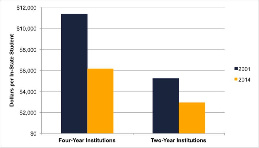
Over the last two decades, state appropriations per undergraduate student have fallen across all public institutions in Virginia, with the reductions over the past ten years having been particularly steep and applicable to every public institution, four-year and two-year alike. Between fiscal years 2001 and 2014, state funding per in-state student declined by 46% and 43% at four-year and two-year institutions, respectively (Figure 2.1).^[27] Compared to reductions in state funding that have occurred in the past, the unique severity of these cuts will likely result in more serious and longer-lasting impacts.

Figure 2.1. State Appropriations per In-State Student

In Virginia, as in most states, state funding for higher education is closely correlated with the strength – and volatility – of the economy. As Figure 2.2 illustrates, cuts in state funding typically take place in the immediate aftermath of a recession. Figure 2.2 shows low points in state funding in the early 1990s (which followed the recession of 1990) and immediately following the recession of 2001, along with the very large cut in funding that resulted from the Great Recession that began in 2007. In the first two cases, we experienced significant upturns in funding as the economy recovered, especially during the prolonged economic expansion of the mid- and late-1990s. The current recession – the Great Recession – appears to be different in important ways, however, and there is reason for concern about current and future levels of state funding even as the state and the nation slowly recover.

Figure 2.2.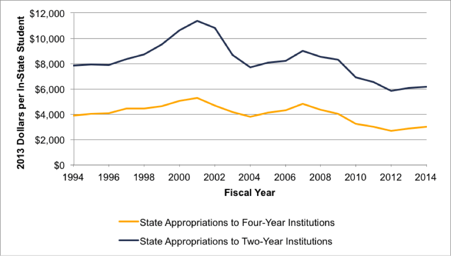

 

The first reason for concern is that the severity of the Great Recession that began in 2007, and the very slow global recovery that has followed, make it unlikely that state funding for higher education will recover as quickly as it did following the 1990 and 2001 recessions. While state appropriations have historically increased as the economy recovered from recessions, the current post-recession economy is far weaker than the economy that followed the 1990 recession. As Figure 2.2 indicates, the lowest levels of state funding resulting from the 1990 recession (which occurred between 1993 and 1995) were still nearly $1,000 per student higher than the level in 2013. Even as Virginia’s economy begins to recover, there are few signs that this recovery will extend to public higher education in the near future. To the contrary, public colleges and universities are facing the strong possibility of continuing reductions in funding.^[28]

Furthermore, the proximity of the last two recessions has compounded their impact on institutional finances, leading to greater total cuts in public funding. While the cuts from the 1990 recession were actually larger (in absolute terms) than those from the 2001 or 2007 recessions, the economy had almost twice as long to recover between 1990 and 2001 as it did between 2001 and 2008. As a result, appropriations per in-state student after the 2001 recession were still 24% lower than their peak levels upon the onset of the 2007 recession. Combining the effects of the two recessions, we saw overall reductions that were larger than those previously experienced and from which there was less time to recover. The result was a decline in funding between 2001 and 2014 that was much larger than the decline after the 1990 recession.^[29]

Finally, large increases in enrollment (particularly since the Great Recession) have placed additional pressures on state resources, driving down funding on a per-student basis and making it less likely that these levels will return to their pre-recession heights. Between 1994 and 2014, four-year and two-year institutions saw a 35% growth in in-state enrollment,^[30] meaning that Virginia would have had to substantially increase funding for higher education in order to maintain per student levels of support.^[31] To be more specific, the state would have had to invest an additional $1.1 billion per year in higher education (equivalent to an 86% increase from its actual level in 2014) to reinstate per-student funding back to its 2001 level. Instead, rather than becoming a funding priority, appropriations to higher education have actually gone down as a fraction of the total state budget, with general fund support dedicated to higher education declining from 14% of the state budget to 11% between 1993 and 2010.^[32]

Institutional Responses to Funding Cuts

While all public institutions in Virginia have experienced declines in state support, they have responded in varying ways. In particular, we noticed significant distinctions between two-year and four-year institutions, as well as among different groups of four-year schools, in terms of their abilities to offset declines in state funding with alternative sources of revenue. The four-year institutions that appear less able to generate new revenue and are therefore more dependent on state funding are referred to in this study as “Higher Dependence on the State” (HDS) institutions. These institutions include: University of Mary Washington, Virginia State University, Christopher Newport University, Longwood University, Old Dominion University, University of Virginia’s College at Wise, Radford University, and Norfolk State University. The four-year institutions that have greater capacities to generate revenue from alternative sources and are therefore less dependent on state funding are referred to as “Lower Dependence on the State” (LDS) institutions.^[33] These include: University of Virginia, College of William & Mary, George Mason University, Virginia Military Institute, Virginia Commonwealth University, James Madison University, and Virginia Tech. In this subsection, we document the strategies adopted by public institutions as a whole and how they differ among these groups of institutions.

State appropriations and tuition revenues have historically constituted the majority of total revenues for most of Virginia’s public institutions of higher education. However, recent declines in public support have forced all of Virginia’s public institutions to become increasingly reliant on tuition revenue in order to balance their budgets. As a result, nearly every institution has raised both its in-state and out-of-state tuition rates, although the magnitude of these increases has varied by institutional type. Institutions have also increased enrollment as a way of increasing tuition revenue, although it is likely that this only increases aggregate revenue from net tuition while actually leading to reductions in revenue per student.^[34] We examine below in more detail how the three types of institutions – LDS, HDS and two-year – responded to declines in state support.

Among LDS institutions, state funding as a share of total revenue dropped from 43% to 23% between 2001 and 2010. Although LDS institutions are able to bring in about 25% of their revenue from sources other than state funding and tuition revenue, they have still seen net tuition revenue as a percent of total revenue increase from 27% to 41% during this time period.^[35] Indeed, increases in tuition rates at LDS schools have occurred for all students, with in-state and out-of-state charges increasing by 107% and 81%, respectively, between 2001 and 2014 (Figures 2.3 and 2.4). Compared to HDS institutions, LDS institutions appear to be better able to generate tuition revenue from both resident and non-resident students, with the absolute increase in in-state tuition among LDS institutions approximately 30% greater than that for HDS schools. In addition, despite the large increases in out-of-state tuition charges, LDS institutions were able to increase out-of-state enrollment by 57% between 2001 and 2014. As we will discuss in more detail below, these two strategies have allowed LDS institutions to offset a greater portion of the state’s funding cuts.

Figure 2.3. Average In-State Tuition and Fee Charges

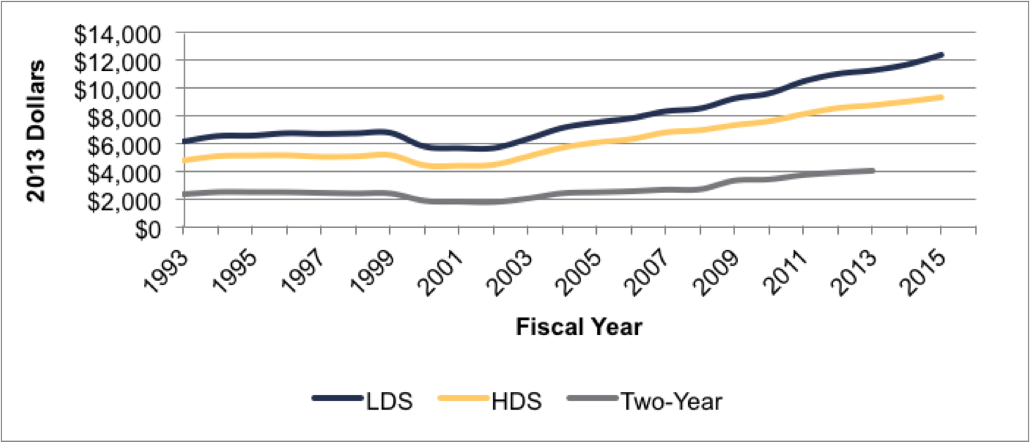
Figure 2.4. Average Out-of-State Tuition and Fee Charges

In contrast with their LDS peers, HDS institutions relied much more on increases in in-state enrollment (which rose by 38% between 2001 and 2014) to grow total tuition revenue. Even though HDS institutions also increased in-state and out-of-state tuition rates appreciably between 2001 and 2014 (by 105% and 61%, respectively), these increases were significantly smaller than those observed by LDS institutions. As a result of these strategies and a decline in public support, the share of total revenue for HDS institutions that came from state funding dropped substantially between 2001 and 2010 (from 56% to 47%). By and large, two-year institutions have also responded to financial challenges in similar ways to the four-year HDS schools – albeit with an even greater reliance on increasing in-state tuition rates and enrollment.

In the midst of these budgetary pressures, four-year institutions as a whole have made considerable investments in financial aid since 2001, with in-state institutional aid as a share of in-state gross tuition rising from 5.9% in 2001 to 13.0% in 2013. However, because this share was very small to start with, the rates of increase would have had to be significantly larger to support more than a small handful of students. Moreover, recent declines in federal and state aid as a fraction of gross tuition have resulted in total aid awarded to in-state students as a share of in-state gross tuition decreasing from 71.1% in 2001 to 69.6% in 2013. In other words, the decreases in the shares associated with state and federal aid have more than canceled out the increases in institutional aid. We will have more to say about the connections between tuition and financial aid in the next section when we address how these institutional decisions affect the net costs that students confront.

Impact on Overall Institutional Financial Structure and Health

Taken together, the data suggest that the three groups of institutions – LDS, HDS, and two-year – relied on somewhat different mixes of strategies in order to increase revenue from net tuition (Table 2.1). LDS institutions relied heavily on higher in-state charges and increases in out-of-state tuition charges and enrollment. HDS institutions – and, to an even larger extent, two-year institutions – instituted increases in tuition charges but also implemented large increases in in-state enrollment. These different approaches have resulted in different implications for institutional finances.

Table 2.1 Changes in Institutional Finances and Enrollment by Institutional Groupings

Average In-State Tuition 2001-2014			Average Out-of-State Tuition 2001-2014		Total In-State Enrollment 2001-2014		Total Out-of-State Enrollment 2001-2014		Average Institutional Gift Aid 2001-2014
	Percentage change from 2001	Average Tuition Charge: 2014	Percentage change from 2001	Average Tuition Charge: 2014	Percentage change from 2001	Total Enrollment: 2014	Percentage change from 2001	Total Enrollment: 2014	Percentage change from 2001	Average Institutional Gift Aid: 2014
LDS	107%	$11,695	81%	$31,433	26%	86,706	32%	25,437	49%	$10,336,165
HDS	105%	$9,070	61%	$21,598	38%	50,639	-25%	5,457	63%	$6,718,312
Two- Year	120%*	$4,088*	56%*	$11,934*	40%	181,660	8%	8,868	583%	$778,241

*Tuition data for two-year institutions are only available up to 2013.

At the risk of underestimating the challenges involved for all institutions, it appears that LDS institutions have been generally successful at offsetting declines in state support, including the large reductions experienced in recent years. Between 2008 and 2014, for example, LDS institutions managed to produce an average increase of 5% per year in combined revenue from tuition and state appropriations per FTE student primarily due to their ability to bring in significant revenue from out-of-state students and maintain high levels of in-state tuition (Figure 2.5). These factors allowed LDS institutions to generate sufficient revenue from tuition to more than offset the loss of state funding without having to resort to large increases in in-state enrollment.^[36]

Figure 2.5. Combined Revenue from Tuition and State Appropriations per FTE Student

HDS institutions, on the other hand, have had much more difficulty maintaining per-student revenue levels. As Figure 2.5 shows, combined revenue from tuition and state appropriations per FTE student declined by an average of 9% between 2008 and 2014, which can be attributed to the rapid expansion of in-state enrollment without comparable increases in out-of-state enrollment or other means of support.

Finally, two-year institutions have been able to offset much of the decline in public funding. In addition to substantial growth in in-state enrollment, they generated a significant amount of revenue by considerably increasing in-state tuition charges. In total, combined tuition and state appropriations revenue per FTE student decreased by an average of only 2% between 2008 and 2014, a result of shifting the cost burden onto in-state students. While perhaps necessary financially, this is worrisome since in-state students are arguably the least able to deal with an increase in charges and most of these institutions have little to no aid to provide for these students.^[37]

Are These Strategies Sustainable?

In the face of current financial challenges, public institutions have largely relied on strategies used in the past. While Virginia’s public institutions have historically been able to successfully offset funding declines through increasing tuition and enrollment, the severity of recent challenges casts doubt on the ability of many of them to keep following these paths. More specifically, tuition charges may be reaching their market limit at many of these institutions, and further increases could both adversely impact institutional finances and endanger the goals of ensuring quality and broad access for students across the state. HDS institutions, in particular, appear to have reached – or at least come close to – this limit, as they were unable to increase tuition charges enough to offset the most recent funding cuts and have thereby seen declines in total revenue per student. And while LDS and two-year institutions have so far been able to institute tuition increases large enough to replace declining state support without a significant market pushback, student demand may not persist if charges continue to rise at such rapid rates.

Indeed, such declines may already be manifesting themselves across the two-year colleges. Table 2.2 illustrates how declines in enrollment have become apparent in two-year institutions over the last few years. If such declines are a sign of price outstripping demand, then four-year and two-year institutions alike may have difficulty in sustaining enrollment and tuition revenues in the future.

Table 2.2. Enrollment and Tuition Changes at Two-Year Institutions

Two-Year Institutions	2008-2010	2010-2011	2011-2012	2012-2013
Number of institutions with decreased enrollment (out of 24)	0	6	12	20
Average percentage change in enrollment (annual)	7%	3%	-1%	-4%
Average tuition increase	13%	9%	5%	3%

Even if the current tuition levels are sustainable from a purely financial perspective, the current reliance on increasing tuition revenue may limit the ability of many institutions to serve their respective missions. In particular, these financial strains may force institutions to choose between sacrificing either access or quality (or some combination of both), particularly for low- and middle-income students. On the one hand, if revenue from tuition increases goes towards filling gaps in the budget left by the declines in state support rather than funding financial aid, the majority of students may see real and substantial increases in the net costs they are expected to pay. On the other hand, if institutions choose to keep tuition low and financial aid high as a way of preserving access for as many students as possible, they will have to think carefully about how to reduce expenditures without sacrificing the quality of the education they provide. Unfortunately, the current funding situation has brought Virginia public higher education to the point of having to make these difficult kinds of choices.^[38]

Section 3: Trends in Net Costs at Four-Year Institutions

We now examine how the changes in the institutional- and state-level financial trends have led to changes in the first-year net costs that students pay to attend a public institution of higher education in Virginia. We use a student-level dataset obtained from SCHEV that contains longitudinal background and financial data for 1,450,321 million students who entered a Virginia public institution of higher education between the 1997 and 2012 academic years.^[39] For a more detailed description of the data and the methodology employed, see Section A.1 of the Appendix.

In this section, we look at in-state, first-time freshmen entering a Virginia public four-year institution on a full-time basis between the 1997 and 2012 academic years, concentrating especially on those who have entered since the beginning of the Great Recession in 2007. Minor adjustments to our sample (due to complications in the data) are described in the footnotes and in greater detail in the Appendix.^[40] We focus primarily on how net costs have changed for poor and near-poor students, using the highest-income students as the main point of comparison. We define net cost as the difference between a student’s total budget for an academic year and the total amount of gift aid (including need-based grants and merit aid) received for that year.^[41] All dollar values are adjusted for inflation and reported in 2013 dollars.

Trends in Average Net Costs

We chose to define our student cohorts based on state-wide income quintiles, designating poor, near-poor, and highest-income students as those who come from families with incomes in the 1^st (lowest), 3^rd (middle), and 5^th (highest) income quintiles in Virginia, respectively.^[42] Defining socioeconomic subgroups in this way allows us to categorize these groups based on objective characteristics of the state’s population. For a sense of what these quintiles look like, Table 3.1 breaks them down by their income ranges for 2012 and their median income levels within our sample of interest.^[43]

Table 3.1. Family Income by Income Quintile (2013 Dollars)

	2012 Income Range	Median for Sample
1st Quintile	$0 - $25,320	$14,912
2nd Quintile	$25,321 - $49,795	$39,526
3rd Quintile	$49,796 - $76,000	$65,839
4th Quintile	$76,001 - $120,670	$101,996
5th Quintile	$120,671+	$165,890

Figure 3.1 illustrates the trends in average net costs between 1997 and 2012 for each income quintile at public four-year institutions in Virginia. We observe that net costs have increased at rates above inflation for nearly every group between 1997 and 2012, with these increases accelerating and becoming more consistent since 2007.^[44] Prior to 2007, the increase in net costs had been greatest – and most steady – for the near-poor and highest-income students, while net costs actually decreased slightly on an average annual basis for students in the lowest income quintile (Table 3.2).^[45] However, after 2007, net costs grew fastest for the poorest students (at an average annual rate of 3.5%) and more slowly for the highest income students – a reversal of the pattern previously observed.

before 2007.^[46] This recent growth in net costs for the poor – and, to a slightly lesser extent, the near-poor – was driven primarily by large increases in these costs from 2010 to 2011, when net costs grew at annual rates of 12.8% and 7.4% for the poor and near-poor, respectively. Moreover, the compounding effect of the Great Recession can be discerned most clearly for near-poor students, for whom net costs in 2006 began to increase even before they were able to fully recover to pre-recessionary levels following the effects of the 2001 recession.

Figure 3.1. Changes in Net Costs over Time

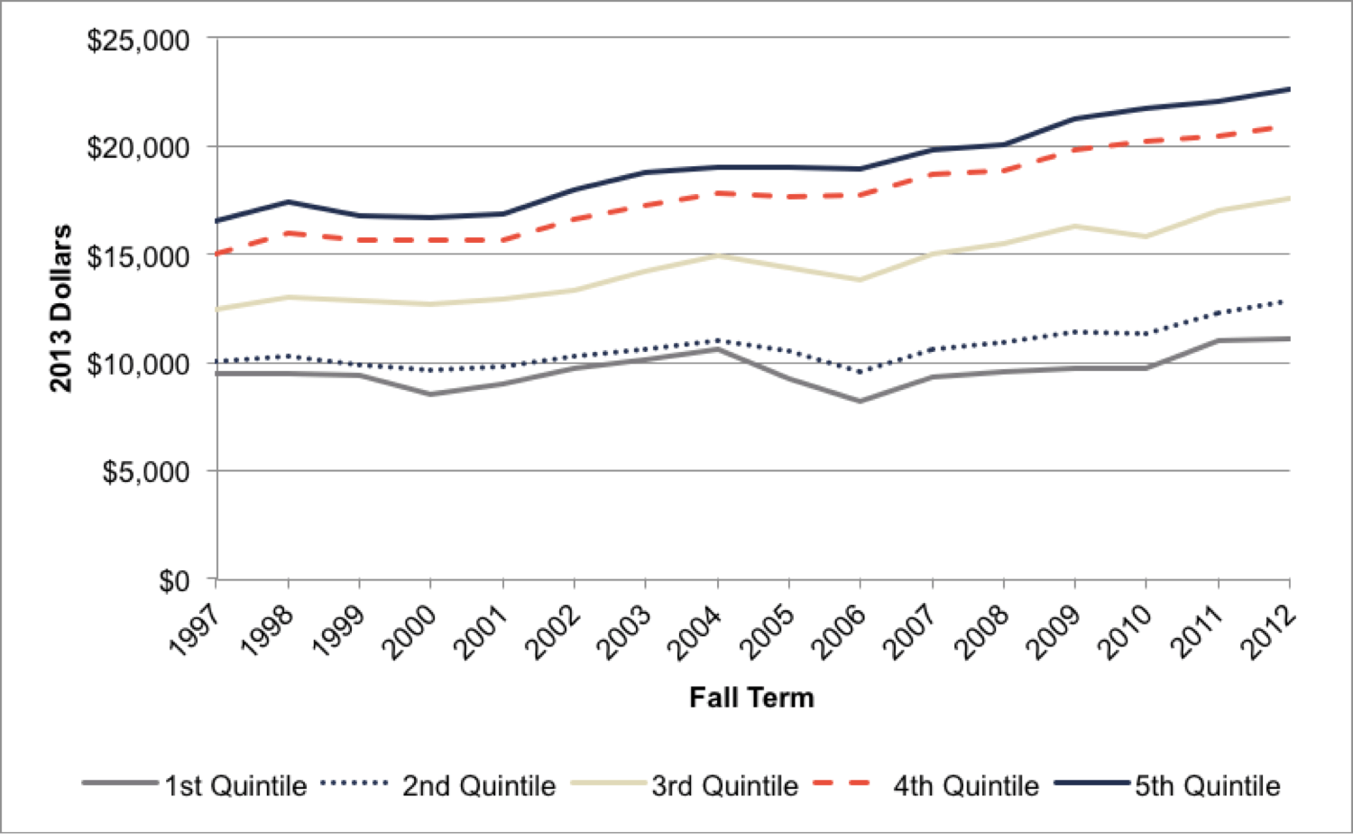
Table 3.2. Annual Rates of Change in Net Costs by Income Quintile

	Poor (1st Quintile)		Near-Poor (3rd Quintile)		Highest-Income (5th Quintile)
1997-98	0.3%	1997-00 Annual Average:-3.5%	4.3%	1997-00 Annual Average:0.7%	5.6%	1997-00 Annual Average:0.3%
1998-99	-0.8%		-1.0%		-4.0%
1999-00	-9.7%		-1.0%		-0.4%
2000-01	5.4%	2000-07 Annual Average:1.2%	1.3%	2000-07 Annual Average:2.4%	1.1%	2000-07 Annual Average:2.5%
2001-02	7.9%		3.7%		6.7%
2002-03	4.2%		6.1%		4.3%
2003-04	4.8%		5.2%		1.6%
2004-05	-13.0%		-3.5%		-0.3%
2005-06	-11.4%		-3.9%		-0.4%
2006-07	14.0%		8.6%		4.7%
2007-08	2.8%	2007-12 Annual Average:3.5%	3.0%	2007-12 Annual Average:3.2%	1.1%	2007-12 Annual Average:2.6%
2008-09	1.9%		5.6%		6.0%
2009-10	0.04%		-3.1%		2.3%
2010-11	12.8%		7.4%		1.8%
2011-12	0.5%		3.3%		2.2%
2001-12 (Average)	1.0%		2.3%		2.1%

Since 2007, the growth in net costs has also outpaced growth in family incomes for students in all income quintiles, with the exception of those in the highest quintile (Figure 3.2).^[47] By 2012, net costs for the median poor and near-poor student constituted 69% and 27% of their respective annual family incomes, while the comparable burden of net costs comprised only 13% of family income for the median highest-income student. These patterns may explain why student borrowing is so prevalent among students in lower income subgroups. Indeed, Figure 3.3 shows that poor students and near-poor students since 2007 have been taking out loans to finance on average 49% and 40%, respectively, of their annual net costs, (contrasted with pre-2007 rates of 39% and 33%). Given the increasing reliance on loans that have accompanied the increases in net costs since the Great Recession, there is ample reason to be worried about how these financial burdens will influence student outcomes over time.

Figure 3.2. Median Net Costs as Percentage of Family Income

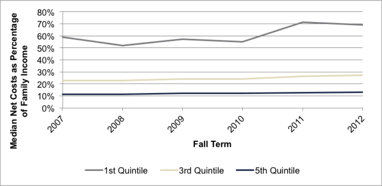
Figure 3.3. Average Loans as Percentage of Net Costs

In summary, we find clear evidence that net costs at Virginia’s public four-year institutions have grown significantly for poor and near-poor students since 2007 (in comparison to both previous years and the rates experienced by their highest-income peers), with these increases accelerating in the most recent years. Furthermore, we find that these patterns persist even after defining student subgroups in different ways (see Section A.1 of the Appendix). These inflation-adjusted increases have, in turn, placed greater financial burdens on those poor and near-poor students and families already struggling to afford a public college education. In later sections, we will examine how these burdens may be influencing student progress towards a degree.

Differences in Trends across Institutions

Next, we disaggregate the net cost trends at the institutional level. Our goal here was not to understand all of the nuances associated with changes at each institution, but rather to confirm that the average trends we observed were prevalent across the entire system and not driven by only a few institutions. Indeed, we found – albeit to varying degrees and with slightly different patterns – that significant increases in net costs for poor and near-poor students have occurred since 2007 at almost every institution.

Figures 3.4a and 3.4b illustrate the respective trends in net costs for poor and near-poor students at each institution since 2007, overlaid by the average trends that we showed earlier. Net costs have increased for poor and near-poor students at almost every institution during this time period, with only a few outliers. While the patterns for poor students seem slightly more scattered, Table 3.3 indicates that these patterns have also begun to converge in the most recent years.^[48] The patterns for near-poor students appear to be more clustered, and Table 3.3 confirms yet again that these trends did not significantly diverge even as net costs continued to increase. Thus, we find evidence that the recent increases in net costs for poor and near-poor students occurred across the entire group of public four-year colleges and universities.

Figure 3.4a. Institution-Level Net Costs for Poor Students

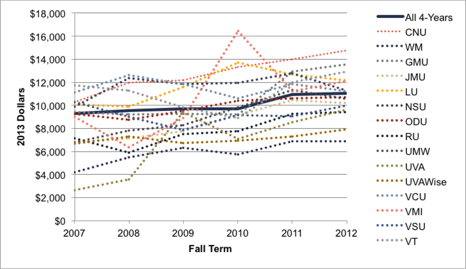
Figure 3.4b. Institution-Level Net Costs for Near-Poor Students

Table 3.3. Standard Deviation between Institutions in Rates of Change for Net Costs

	Poor (1st Quintile)	Near-Poor(3rd Quintile)
1997-2007 (Average)	0.20	0.09
2007-08	0.18	0.09
2008-09	0.15	0.05
2009-10	0.13	0.07
2010-11	0.17	0.13
2011-12	0.07	0.04

Changes in the Components of Net Costs

We now examine how changes in the components of net cost – namely, tuition and various sources of gift aid – have interacted to produce the overall increases in net costs documented thus far. Concentrating on poor and near-poor students since 2007, we carried out this analysis for the set of all four-year institutions, as well as for LDS and HDS institutions separately. Because LDS and HDS schools have attempted to cope with declining state support in somewhat different ways (see Section 2), we were interested in seeing to what extent there exist structural differences between the two groups with regard to whether and how they have shifted the financial burdens onto their students.

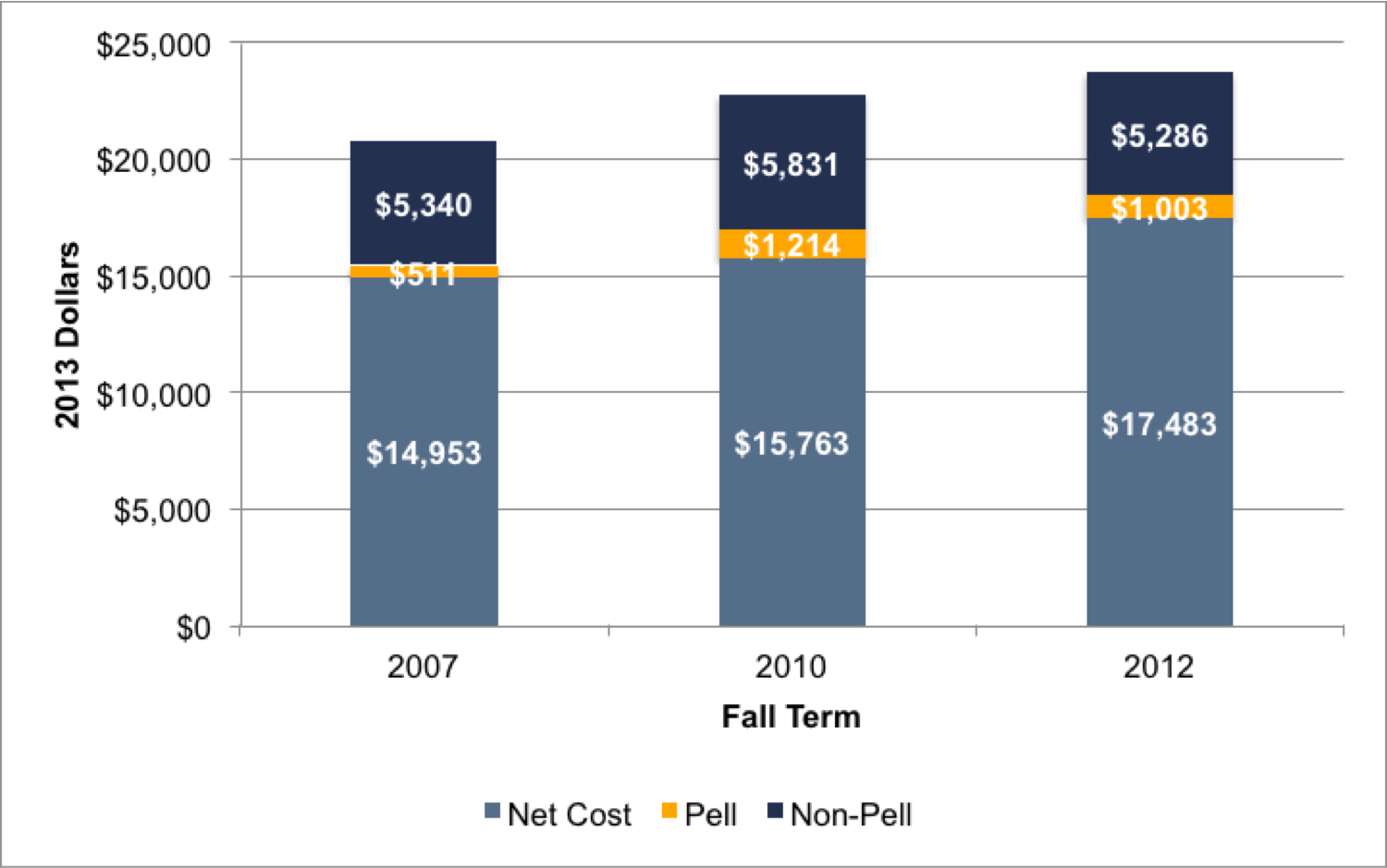
For poor students at all four-year institutions, average net costs grew by less than $400 between 2007 and 2010, a surprisingly modest number given the financial challenges these institutions faced. Figure 3.5a shows that the growth in average gift aid during this time period (spurred by a large increase in the average Pell Grant) was nearly enough to offset the growth in average student charges. From 2010 to 2012, the growth in student charges actually moderated somewhat, but the large reductions in both sources of gift aid (state/institutional aid and Pell Grants) that occurred simultaneously led to the dramatic increase in net costs that we observed in Figure 3.1 and Table 3.2.^[49]

Figure 3.5b tells a similar story for near-poor students across all four-year institutions, with average gift aid rising from 2007 to 2010 but then falling slightly from 2010 to 2012, even as student budgets increased throughout. Note that Pell Grants make up a smaller fraction of total gift aid for near-poor students, who therefore did not benefit from as large an increase in gift aid as poor students did from 2007 to 2010 (when Pell Grants considerably increased in value). Consequently, near-poor students faced a substantial increase in net costs from 2007 to 2010 and an even larger increase from 2010 to 2012 when state and institutional gift aid declined.

Figure 3.5a. Components of Overall Net Costs for Poor Students

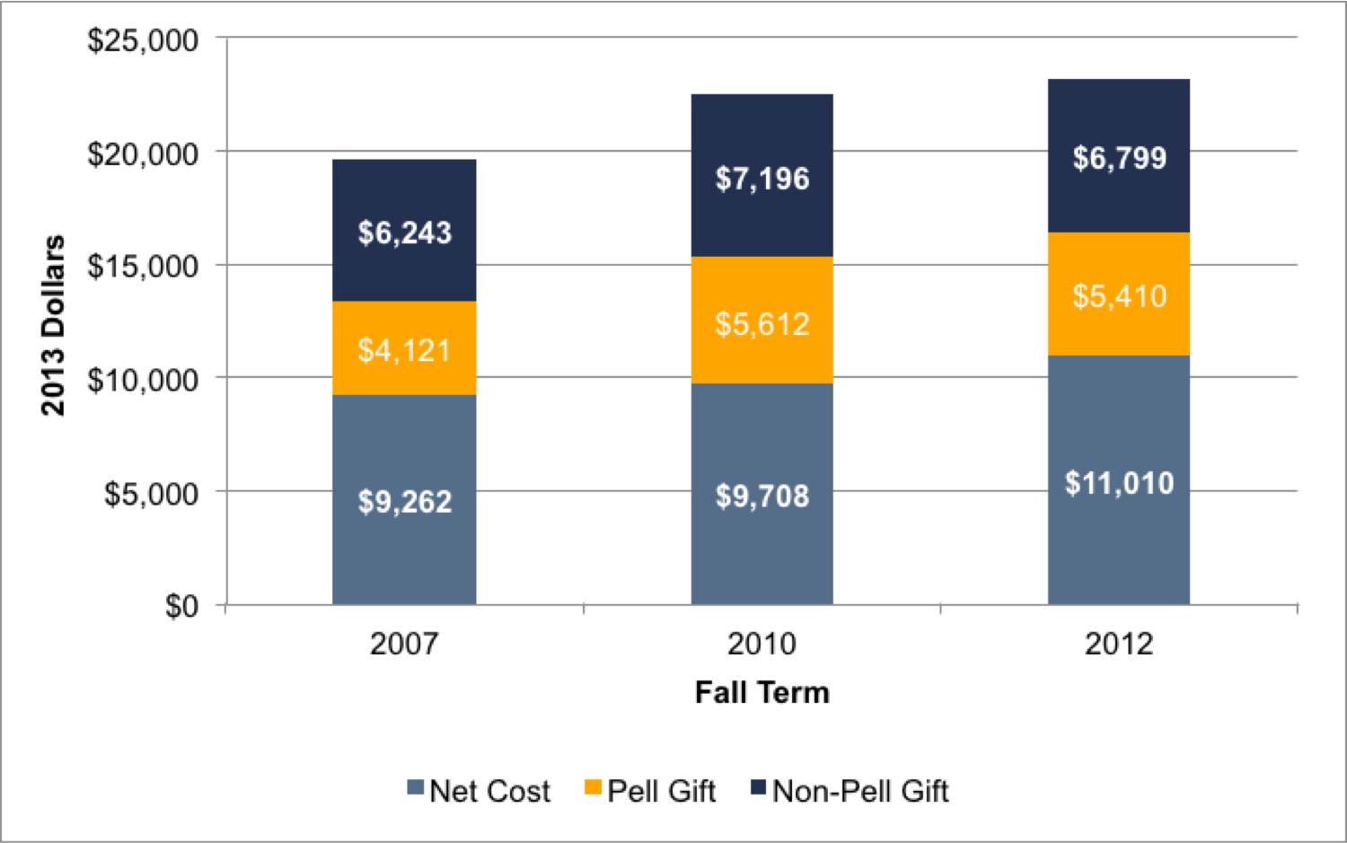
Figure 3.5b. Components of Overall Net Costs for Near-Poor Students

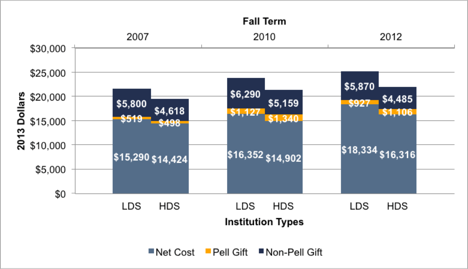
These general patterns seem most intense among LDS institutions, which instituted both larger increases in student charges and saw greater reductions in gift aid between 2010 and 2012 than their HDS peers. Indeed, 2012 marked the first year in which average net costs for poor students in our sample were lower at HDS institutions than at their LDS counterparts, as the traditionally high levels of gift aid at LDS institutions had until recently kept pace with their consistently higher student budgets (Figure 3.5c). Similarly, while net costs have always been greater at the LDS institutions for near-poor students, the difference in net costs between LDS and HDS institutions for the near poor has continued to increase in the most recent years (Figure 3.5d).

Figure 3.5c. Components of LDS and HDS Net Costs for Poor Students

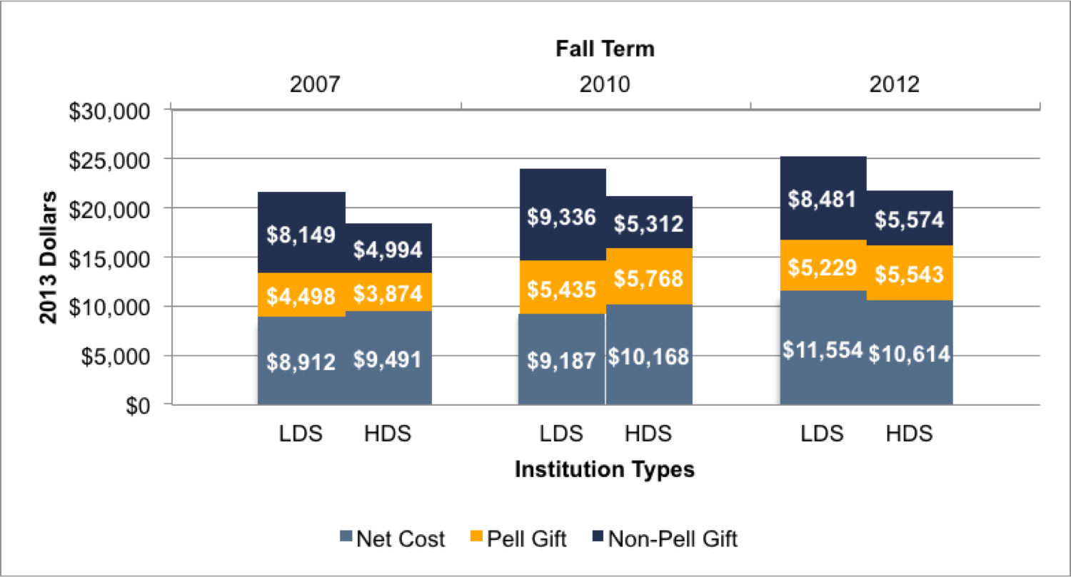
Figure 3.5d. Components of LDS and HDS Net Costs for Near-Poor Students

In summary, student charges have increased significantly faster than inflation at all institutions since 2007, while the growth in financial aid for poor and near-poor students has been slower and less consistent. In particular, the decline in gift aid for these students from 2010 to 2012 resulted in significant increases in net costs that outpaced increases observed in previous years. Because gift aid generally constitutes less than half the amount of student budgets for both poor and near-poor students, financial aid would have had to grow at more than twice the rate of student charges in order to completely offset tuition increases. Anything less – let alone the flattening or declining rates of change for gift aid that occurred in the most recent years – results in an increase in net costs for these students, thus threatening the ability of poor and near-poor students to finance their education. Indeed, we calculated that total financial aid across all four-year institutions would have had to increase by $11.4 million for poor students and $20 million for near-poor students to merely hold the students in our sample harmless just from the increases in student charges between 2007 and 2012.^[50]

The growth in net costs since the onset of the Great Recession, and particularly for the poorest students in recent years, raises questions about how these costs are influencing student decisions to pursue and earn a degree. We hypothesize that the increasing burden that poor and near-poor students and their families must bear in order to finance a post-secondary education may very well impact whether or not these students pursue a four-year degree and how steadily they move towards achieving that degree. In the next section, we look at trends in student enrollment, first-year retention, and four-year graduation rates to see if there are any patterns that may be readily linked to the growth in net costs. In the subsequent section, we employ multivariate regressions to examine more rigorously how net costs are related to student outcomes.

Section 4: Trends in Student Enrollment, Retention, and Graduation

The growth in net costs since 2007, especially for the poorest students, raises important questions regarding how these costs are influencing student decisions to enroll at a public four-year institution, remain enrolled, and complete a degree in a timely manner. In this section, we look at patterns in student enrollment, first-year retention, and four-year graduation between 1997 and 2012 to see if there have been any changes that may be tied to trends in net costs.^[51]

Enrollment

Since 1997, the total enrollment of students in our sample (in-state, first-time freshmen enrolling on a full-time basis at public four-year institutions) has increased at an average rate of 2.5% per year, although this growth rate has slowed slightly since 2007 to an average of 1.5% per year (Figure 4.1).^[52] Figures 4.2 and 4.3 break down the overall enrollment trend by income quintile, with the former showing overall enrollment numbers and the latter indicating enrollment percentages by quintile.^[53] Since 2007, there has been a significant increase in the enrollment of students who filled out FAFSA forms and a corresponding decrease in the number of students who did not fill out a FAFSA. While it is hard to identify cause-and-effect relationships, it appears that the sharp decrease in “No FAFSA” students from 2007 to 2008 occurred simultaneously with a substantial increase in the number of students from the 5^th income quintile who decided to apply for financial aid. Since 2010, however, enrollments across all income quintiles have largely remained flat. As a result, while there are clearly many more factors at work during these years in addition to rising net costs (for example, the improving job market), enrollment among students in the lower-income quintiles has stopped growing and remains well below the enrollment numbers of their higher-income peers.

Figure 4.1. Total Enrollment

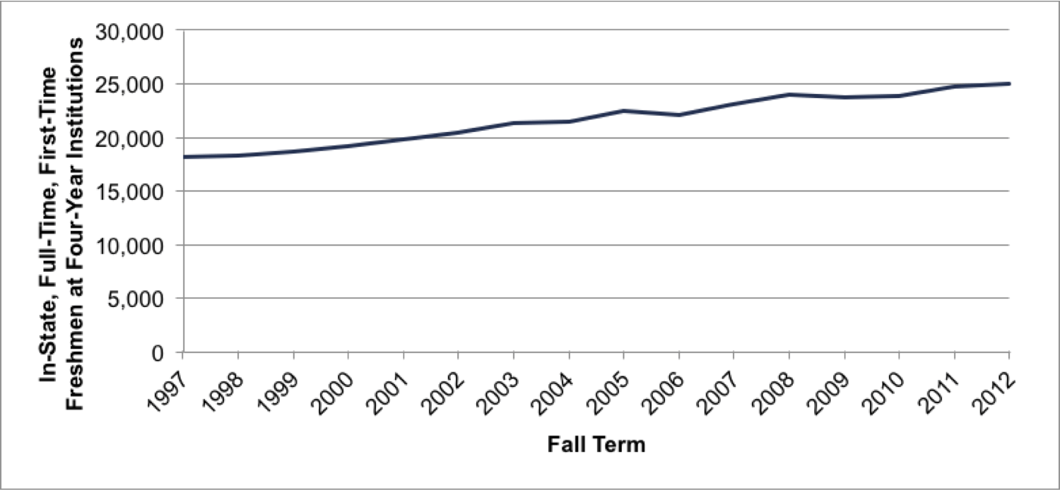
Figure 4.2. Enrollment Numbers by Income Quintiles

Figure 4.3. Enrollment Percentages by Income Quintiles

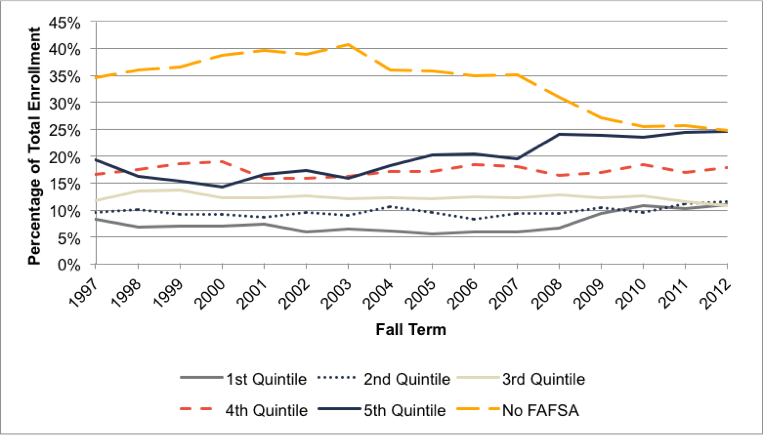
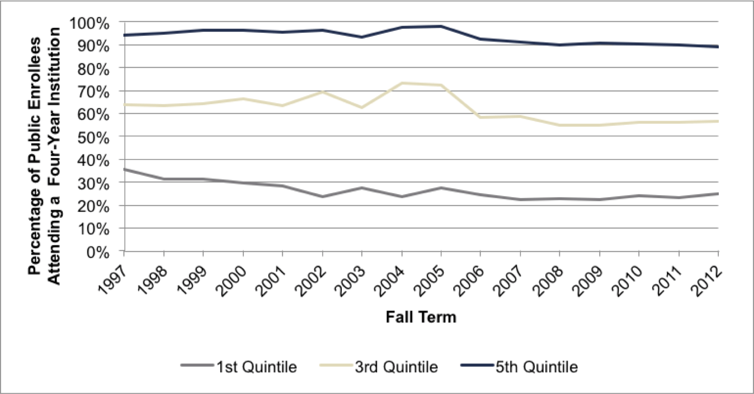
Figure 4.4 frames these enrollment trends in a different – and more troubling – context, showing enrollments among poor, near-poor, and highest-income students at four-year public institutions as percentages of total enrollment among each income subgroup in any public Virginia institution of higher education (public four-year and two-year).^[54] Since 2007, these patterns have remained largely unchanged for all of these subgroups, with approximately 90% of all highest-income and 56% of near-poor public college enrollees in Virginia starting at a four-year institution. This level drops significantly for the poor, for whom only 23% of all public college enrollees since 2007 initially enrolled at a four-year school, with this percentage having steadily declined from a high of 35% in 1997.^[55] These trends suggest that, since 2007, there has been no progress in shrinking the very large socioeconomic gap among entering students in terms of attendance at four-year institutions. Students in the lowest-income quintile – in contrast with their higher-income peers – are still overwhelmingly likely to enroll in a public two-year institution and not a four-year institution.

Figure 4.4. Enrollment at Four-Year Institutions as Percentage of Total Statewide Enrollment

Relatively few students who start at a two-year institution earn an associate’s degree, and even fewer transfer to a four-year institution and ultimately earn a four-year degree.

This is particularly troubling since success rates are much lower for students who start at a two-year school compared to those who start at a four-year school – even for those who enroll on a full-time basis. As Table 4.1 indicates, relatively few students who start at a two-year institution earn an associate’s degree, and even fewer transfer to a four-year institution and ultimately earn a four-year degree. If differences in net costs push large numbers of students to attend two-year institutions instead of four-year institutions, there is a significant reason to be concerned about these students’ prospects for earning a bachelor’s degree. If we are to make progress in increasing the overall number of college graduates and narrow the existing gaps between socioeconomic groups, it is important to both address the costs of earning a degree and raise the success rates of students attending community colleges.

Table 4.1. Success Measures by Original Institution Type and Full-Time Status

	Retained for a Second Year	Earned a Bachelor’s Degree in 4 Years	Earned a Bachelor’s Degree in 6 Years	Earned an Associate’s Degree in 2 Years	Earned an Associate’s Degree in 3 Years	Transferred to Four-Year Inst. within 2 Years	Earned an Associate’s or Transf. to a Four-Year Inst. within 3 Years
Four-Year Full-Time	84%	42%	66%
Four-Year Part-Time	67%	27%	39%
Two-Year Full-Time	54%	2%	5%	5%	12%	5%	18%
Two-Year Part-Time	37%	3%	4%	3%	7%	3%	10%

Retention Rates

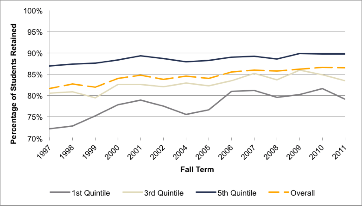
We find similar patterns in student progress towards a degree. Overall first-year retention rates among first-time, full-time students at public four-year institutions have increased slightly since 1997 but have hovered around an average of 85% (Figure 4.5). The breakdown by income quintiles shows that the highest income students are on average 11 percentage points more likely to be retained than the lowest income students, and 6 percentage points more likely than students in the 3^rd income quintile. Thus, even among the few low-income students who begin as full-time students at 4-year institutions, the chances of persisting are less than those of their higher-income peers.

We see similar trends for first-year persistence (which includes all students who were retained or transferred), though the rates are slightly higher (91%) because transfer students are counted as persisting. Of the 15% of students who are not retained after the first year, approximately 40% transfer, 29% drop out, and 31% take time off.^[56] These shares have remained relatively stable over this period as well.

Figure 4.5. First-Year Retention Rates

Four-Year Graduation Rates

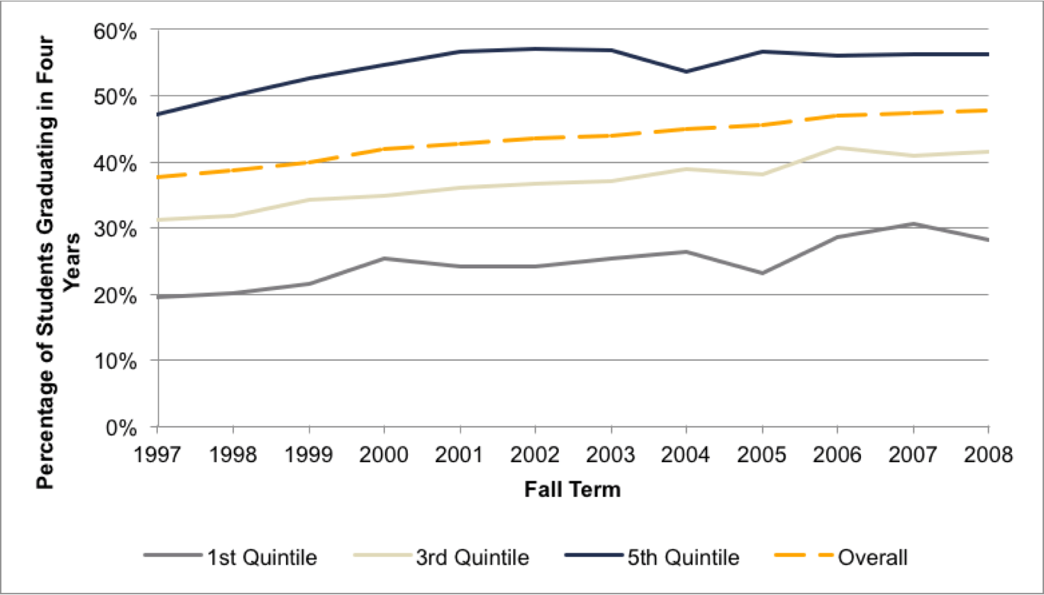
The overall four-year graduation rate has been increasing since 2001, from 37% for the cohort that entered in 1997 to 48% for the cohort that entered in 2008. While these increases have occurred for both the lowest and highest income groups, it is important to note that the gap in graduation rates between the 1^st and 5^th income quintiles has not closed over time and has instead held roughly stable at about 30 percentage points per year (Figure 4.6). Indeed, this gap was 28 percentage points for both the cohort entering in 1997 and the cohort entering in 2008. This strongly suggests that we have fallen well short of achieving the stated goal of “equal opportunity for all” throughout this period. While we do not have graduation rate data for later cohorts, there is little reason to believe that progress has been made since 2008. In fact, the data on retention rates and other success measures suggest that, if anything, we are headed in the opposite direction.

Figure 4.6. Four-Year Graduation Rates

While we do not see significantly worsening trends in student outcomes and enrollment in light of rising net costs since 2007, it is clear that the current levels are not improving at the rate they would need to in order to achieve national and state goals for higher education. This is especially true for low-income students, who are significantly less likely to enroll at four-year institutions in the first place, and also less likely to re-enroll for a second year. We fear that the increases in net costs we have seen – and expect to continue seeing – will further reduce these students’ likelihood of success. We test this hypothesis in our next section, where we employ regression methods to examine how increases in net costs – holding other factors constant – are related to changes in student retention, persistence, credit completion, and graduation.

Section 5: Descriptive Analysis of the Impact of Rising Net Costs on Student Success

Against the backdrop of continuing growth in net costs, this section presents the results of multivariate regression analyses designed to determine the extent to which the increases in net costs have affected student patterns in enrollment and degree completion.^[57] These regression techniques hold constant a variety of student characteristics, in addition to controlling for institution- and year-fixed effects. Using first ordinary least squares (OLS) regression techniques, we find that net costs are negatively related to student re-enrollment at the same or another institution after the first year, the number of credits completed, progress towards a four-year degree, and graduation in four years. These effects are statistically significant and largest for the poorest students, who have also seen the fastest growth in net costs since 2007 and have the lowest retention and graduation rates to begin with.

We will report in the next section on a difference-in-differences quasi-experiment which exploits an exogenous change in expected family contribution (EFC) rules for certain low-income students to estimate the causal impact of a reduction in net costs on the success rates of those students. In that analysis, we find that a decrease in net costs has an even larger inverse effect on first-year retention than the effects we calculate via the OLS methodology. Taken together, these two sets of findings strongly suggest that the cumulative effect of continuing growth in net costs, holding other factors constant, will result in a substantial decline in student success rates and a further widening of the gap between success rates for students from different socioeconomic groups.

Methodology

For the OLS analysis, we examined a subset of the sample of first-time, full-time students at public four-year institutions that we analyzed in the previous sections. In particular, we limited our sample to those students who enrolled for an entire year and who entered in the fall term in order to ensure that we have accurate financial data for all students in our analysis. We also limited our sample to students who enrolled during and after 2004, since these are the only years in which data for SAT scores (which are needed to control for different levels of student preparedness) were collected. Finally, we dropped from our sample those students who did not file a FAFSA or who were missing EFC information.

In this section, we subdivided students based on their levels of EFC instead of income quintiles, given some complications with the income data and because EFC is the official metric used to determine a student’s gift aid. When not addressed, the potential errors in the income data (which include a number of students having low incomes and high EFCs or very different incomes between years) could bias the standard errors in our regressions and thus compromise some of our results. The greater reliability of the EFC data lends more credibility to the analysis of net costs and student outcomes when we break down the results by groups. However, it is important to note that these complications in the income data only appear to affect the student-level analyses done in this section and should not significantly bias the trends averaged across students reported in the previous sections. Indeed, the mean trends in net costs, enrollment, and outcomes for the EFC groups and income quintiles follow virtually identical patterns.^[58]

Students are classified into four EFC quartiles based on the distribution within each year of first-year EFC levels for all students who entered a Virginia institution. The 1^st EFC quartile is entirely composed of students with zero EFC and looks similar to the poor or low-income students referred to in previous sections. We characterize the 2^nd EFC group as near-poor, and the 3^rd and 4^th quartiles as higher-income. Table 5.1 describes these groups in the context of their income distributions, with additional explanations of this classification method available in Section A.1 of the Appendix.

Table 5.1. Description of Income Levels by EFC Quartile

Percentile within the EFC Quartile	EFC Q1	EFC Q2	EFC Q3	EFC Q4
1%	$0	$0	$0	$0
25%	$3,948	$26,374	$50,262	$102,635
50%	$14,090	$38,474	$69,013	$132,790
75%	$24,507	$48,920	$86,116	$175,136
99%	$69,099	$83,851	$147,523	$480,789

We employed a few different regression models in order to better understand the relationship between net costs and student success. We started with OLS regressions for our key outcome variables (first-year retention, first-year persistence, credits earned, progress towards a degree, and four-year graduation). In order to see how net costs influence these different measures of student success (holding all other factors constant), we included controls for student characteristics – including income at entry, EFC at entry, age, race, gender, SAT score, unemployment rate in the home zip code, campus housing status, and dependent status – as well as institutional- and year-fixed effects.^[59] We then estimated regressions using both linear and non-linear specifications on net cost to see if students respond in different ways depending on their level of net cost, and we conducted a few robustness checks with different samples of the data. Next, we turned to a hazard model using a multinomial logistic regression, which enables us to compare all possible outcomes at the end of year one, as well as how net costs are associated with each path that a student can take (re-enrolling at the same institution, enrolling at another institution, and not persisting).^[60]

Results

Table 5.2 presents the OLS regression results for first-year retention and first-year persistence, both of which are binary variables indicating whether or not a student was retained (at any institution) or persisted (at the same institution). The coefficients displayed denote the effect of an additional thousand dollars in net costs on student retention and persistence and represent changes in percentage points. The bottom line is that increases in net costs for each EFC quartile have a statistically significant, negative impact on student success.

Net costs have the largest impact on the poorest students. A $1,000 increase in net costs is associated with a 0.63 percentage point reduction in the likelihood of re-enrolling at any institution in the second year for students in the 1^st EFC quartile (representing a reduction in the probability of being retained from 78.38% to 77.75%). While this effect appears small, it is statistically significant at the 99% confidence level – meaning that we can be 99% confident that the impact of increasing net cost is negative – and the cumulative effect of continuously rising costs can become large over time. Moreover, this result comes at a time when the goal is to reduce – not to increase – the gaps across subgroups.

We also look at first-year persistence rate (re-enrolling at the same institution) to ensure that the previous effect is not entirely driven by transfer students. For students in the 1^st EFC quartile, a $1,000 increase in net costs reduces the probability of persisting into the second year by 0.54 percentage points. The effects decrease in magnitude for higher quartiles, but the coefficients on net costs are still negative and statistically significant at the 99% level for all four EFC quartiles. This suggests that, if net costs continue to increase at the rates we observed in Section 3, student retention and persistence rates will suffer – especially among the most disadvantaged students.

Table 5.2. Impact of a $1,000 Increase in Net Costs on First-Year Retention and Persistence

	First-Year Retention	First-Year Persistence
	$1,000 in Net Cost
EFC Q1	-0.00631***	-0.00537***
	(0.00088)	(0.00075)
EFC Q2	-0.00472***	-0.00357***
	(0.00085)	(0.00069)
EFC Q3	-0.00446***	-0.00280***
	(0.00061)	(0.00045)
EFC Q4	-0.00249***	-0.00142***
	(0.00038)	(0.00024)
Clustered standard errors are in parentheses. *** p<0.01, ** p<0.05, * p<0.1. All regressions control for income at entry, expected family contribution at entry, age, race, gender, SAT score, unemployment rate in home zip code, living on campus, and dependent status. They also include dummy variables for each year and institution fixed effects.

The smaller coefficients for the higher EFC quartiles may be partly due to the fact that $1,000 constitutes a smaller portion of their total net costs. Thus, we reviewed the regression results using logged net costs to examine the effect associated with a 1% increase in net costs. These results are displayed in Table 5.3 and show similar patterns as the results in Table 5.2, although the effects of increasing net costs are now larger for the 3^rd and 4^th EFC quartiles. This makes sense given that a 1% increase in net costs is larger in magnitude for these students (with a 1% increase in net costs for the 4^th quartile constituting $204, compared to $91 for the 1^st quartile).^[61] Once again, we find that net costs have a statistically significant and negative impact across the board on student success.

Table 5.3. Impact of a 1% Increase in Net Costs on First-Year Retention and Persistence

	First-Year Retention	First-Year Persistence
	1% increase Net Cost
EFC Q1	-0.03516***	-0.02899***
	(0.00586)	(0.00432)
EFC Q2	-0.02136***	-0.01727***
	(0.00531)	(0.00360)
EFC Q3	-0.05769***	-0.03648***
	(0.00768)	(0.00524)
EFC Q4	-0.03737***	-0.02057***
	(0.00648)	(0.00365)
Clustered standard errors are in parentheses. *** p<0.01, ** p<0.05, * p<0.1. All regressions control for income at entry, expected family contribution at entry, age, race, gender, SAT score, unemployment rate in home zip code, living on campus, and dependent status. They also include dummy variables for each year and institution fixed effects.

Other Measures of Student Success

We also looked at other indicators of first-year success and how net costs impact them. These results are presented in Table 5.4. We find that each additional $1,000 in net costs significantly reduces the number of credits earned in a student’s first year by 0.21 credit hours for students in the 1^st EFC quartile. Some of this is due to these students attempting fewer credits, as a $1,000 increase in net costs reduces the number of credits attempted in year one by 0.051 credits. Thus, if we control for credits attempted in the credits earned model, we see that the effect on credits earned is reduced to -0.15 credits. Although these estimates are small, as we indicated above, the overall impact of rising net costs on an individual student’s chances of success are larger than that – students looking at rising costs are pushed to both take fewer credits and are less likely to complete the credits they do take.

Similarly, net costs reduce the rate of progress students make towards a four-year degree.^[62] However, it is less clear what impact net costs have on the four-year graduation rate. The overall impact of net costs on the four-year graduation is statistically significant at the 95% confidence level when estimated across all students, and it is significant at the 99% confidence level within each EFC quartile. Although the effect is actually larger for the 2^nd and 3^rd quartiles than for the 1^st and 4^th, the effects across all quartiles are still relatively small.^[63]

Table 5.4. Impact of $1,000 Increase in Net Costs on Additional Indicators of Student Success

	Credits Attempted Year 1	Credits Earned Year 1	Credits Earned Year 1, controlling for attempted credits	Progress Year 1	Graduate in 4 years
EFC Q1	-0.05081***	-0.20700***	-0.14825***	-0.00686***	-0.00703***
	(0.01098)	(0.02148)	(0.01837)	(0.00071)	(0.00174)
EFC Q2	-0.05330***	-0.17520***	-0.11609***	-0.00561***	-0.00847***
	(0.00884)	(0.02129)	(0.01679)	(0.00069)	(0.00171)
EFC Q3	-0.05055***	-0.10819***	-0.05214***	-0.00321***	-0.01117***
	(0.00609)	(0.01598)	(0.01513)	(0.00055)	(0.00134)
EFC Q4	-0.04141***	-0.07018***	-0.02572*	-0.00202***	-0.00579***
	(0.00683)	(0.01824)	(0.01472)	(0.00058)	(0.00115)
Clustered standard errors are in parentheses. *** p<0.01, ** p<0.05, * p<0.1. All regressions control for income at entry, expected family contribution at entry, age, race, gender, SAT score, unemployment rate in home zip code, living on campus, and dependent status. They also include dummy variables for each year and institution fixed effects.

Thus, while all of our results find relatively small relationships to date between outcome indicators and net costs, these relationships are statistically significant at the 99% confidence level for all EFC quartiles in all but three cases, and are negative in all cases. The consistency of these results and the variety of outcomes we explored suggest that rising net costs do indeed have a statistically significant, negative effect on efforts to improve student outcomes. Consequently, if net costs continue to grow at rates similar to those Virginia has experienced since 2007, then we can only expect the sobering result that student success rates are very likely to decline.^[64]

Supporting Evidence

While we control for student characteristics at entry and for institutional- and year-fixed effects in our OLS specifications, there may still be some unobservable student characteristics (such as intrinsic motivation) and institutional factors (such as policy changes) that affect these outcomes. While the large size and diversity of our population reduce some of the concerns about threats to internal validity, our confidence in these results is bolstered by their consistency across indicators and with previous research.^[65] Nevertheless, we chose to conduct additional robustness checks on our original results in order to be as thorough as possible.

We examined the results from a hazard model to more precisely estimate the impact of net costs on each path that a student can take at the end of his/her first year. The results in Table 5.5 show how a $1,000 increase in net costs is related to the probability that a student follows a certain path at the end of year one (compared to the baseline path of remaining enrolled).^[66] We see that all non-reenrollment paths are positively and significantly related to higher net costs, with a $1,000 increase in net costs associated with a student being 1.06 times as likely to not persist (by dropping out or taking time off).^[67] Net costs do not have a statistically significant impact on whether or not students in the 1^st EFC quartile transfer, although they do have a significant impact on the transfer patterns for students in the 2^nd and 3^rd EFC quartiles (with students in the 3^rd EFC quartile being 1.04 times as likely to transfer given an increase in net costs of $1,000). These results also show that net costs are more related to persistence (rather than transfer) patterns for the separate EFC quartiles.

Table 5.5. Relative Risk Ratios of a $1,000 Increase in Net Costs on Not Persisting and Transferring, Compared to Remaining Enrolled after Year 1

	Not Persisting	Transferring
EFC Q1	1.06172***	1.01988
	(0.00966)	(0.01276)
EFC Q2	1.06146***	1.02337*
	(0.01109)	(0.01226)
EFC Q3	1.06121***	1.03902***
	(0.00939)	(0.00961)
Clustered standard errors in parentheses and *** p<0.01, ** p<0.05, * p<0.1. All regressions control for income at entry, expected family contribution at entry, age, race, gender, SAT score, unemployment rate in home zip code, living on campus and dependent status. They also include dummy variables for each year and institution. Not persisting includes dropping out and/or taking time off.

Furthermore, we tested additional non-linear forms of the relationship between net costs and student outcomes to confirm that our linear model provided the best functional form to estimate these effects. First, the addition of a quadratic term for net cost did not alter our results. In addition, the results using the natural log of net costs presented earlier display similar results to those of the linear specification. We also found similar results using logistic and probit regression models, with these results are all presented in Section A.2 of the Appendix.

It is possible that there are some groups of students or institutions for whom the effects may differ. To determine whether this is true in our case, we disaggregated our overall sample in several different ways (Table 5.6). First, we limited the sample to only dependent students, since they have different financial resources and aid calculations than independent students. Since the overwhelming majority of our sample is comprised of dependent students, dropping the independent students does not significantly change the results.^[68] Second, some prior research has found that female outcomes are more sensitive to financial aid than those of males, so we estimated separate regressions by gender.^[69] Here, we found slightly larger effects for male first-year retention rates, although net costs had a larger impact for female graduation rates. The impact of net costs also appears to be slightly larger for minority and low-SAT students. While the differences between student groups are not huge in most cases, the effects appear to be somewhat larger for the populations that are most typically disadvantaged in educational settings and may already be less likely to persist or graduate. This adds emphasis to our concern that changes in net costs are limiting the effectiveness of ongoing efforts to improve student success rates within Virginia’s public institutions and may very well exacerbate the current gaps in student outcomes among these groups. In other words, regardless of how we conduct the tests and carry out the descriptive analyses, it seems very clear that students who are disadvantaged in various ways as they enter college are disproportionately impacted by rising net costs.

We also estimated separate regressions based on the two groups of schools identified earlier in the report – High Dependence on the State (HDS) and Low Dependence on the State (LDS). We found larger impacts for the HDS schools than the LDS Schools for first-year retention, first-year persistence, and four year graduation. This is probably due to the differences in student bodies, since the HDS schools are composed of a higher proportion of lower-income, lower-SAT, and minority students, for whom we find larger associations between net costs and student outcomes. While HDS schools have actually seen a smaller growth in net costs than LDS schools, there is concern that the continuing budget pressures and a growing need for tuition revenues may eventually produce seriously adverse effects on HDS students.

Table 5.6. Impact of $1,000 Increase in Net Cost by Subgroups

	First-Year Retention		Four-Year Graduation
	EFC Q1	EFC Q3	EFC Q1	EFC Q3
Overall	-0.00631***	-0.00446***	-0.00703***	-0.01117***
	(0.00088)	(0.00061)	(0.00174)	(0.00134)
Dependent	-0.00631***	-0.00452***	-0.00794***	-0.01119***
	(0.00092)	(0.00061)	(0.00178)	(0.00135)
Female	-0.00578***	-0.00321***	-0.00950***	-0.01144***
	(0.00103)	(0.00061)	(0.00222)	(0.00189)
Male	-0.00701***	-0.00631***	-0.00306	-0.01047***
	(0.00132)	(0.00102)	(0.00252)	(0.00138)
Minority	-0.00799***	-0.00387**	-0.01011***	-0.00872***
	(0.00140)	(0.00149)	(0.00199)	(0.00250)
High SAT	-0.00499***	-0.00430***	-0.00215	-0.01090***
	(0.00139)	(0.00089)	(0.00331)	(0.00177)
Low SAT	-0.00729***	-0.00468***	-0.00941***	-0.01165***
	(0.00106)	(0.00102)	(0.00169)	(0.00190)
HDS	-0.00720***	-0.00665***	-0.00781***	-0.01563***
	(0.00139)	(0.00120)	(0.00208)	(0.00226)
LDS	-0.00567***	-0.00306***	-0.00623**	-0.00838***
	(0.00102)	(0.00059)	(0.00282)	(0.00154)

Section 6: Causal Analysis – A Difference in Differences Quasi-Experiment

In order to test more robustly the causal link between net costs and student success rates, we exploit a quasi-experiment embedded in our dataset through a difference-in-differences research design. Doing so allows us to examine the causal relationship between net costs and first-year retention in a particular setting and assess this result in the context of the OLS results presented in Section 5. While this method necessarily ties us to the particular event from which the quasi-experiment arose, it allows us to investigate the relationship between net costs and first-year retention free of the confounding factors that may have the potential to bias our previous results. In the end, the combination of the difference-in-differences and OLS results adds greatly to our confidence that rising costs have had a statistically significant, negative effect on student success, and one that is especially adverse for the poorest students.

The Experiment

As part of the College Cost Reduction and Access Act of 2007, the federal government agreed to increase the income threshold required for an automatic zero expected family contribution (EFC) from $20,000 to $30,000.^[70] This policy change officially went into effect during the 2009-10 academic year. Calculated from responses on the FAFSA, a student’s EFC is the official determinant of a student’s financial need and establishes a student’s eligibility for a number of federal, state, and institutional aid programs. In addition to meeting the income threshold, a student’s household seeking to qualify for an automatic zero EFC must also have received benefits from a means-tested Federal benefit program, and/or have parents who either filed certain tax forms, were exempt from filing income tax returns, or were dislocated workers.^[71] While a student does not necessarily have to meet these conditions to ultimately receive a zero EFC (as there are other factors that affect a student’s financial aid award), relaxing these conditions makes it “easier” for more students to obtain access to greater amounts of need-based aid.

As Figure 6.1 shows, the increase in the income threshold from 2008 to 2009 was the largest single-year increase between 2001 and 2014.^[72] Given that this was an exogenous policy change uncorrelated with student-level characteristics, we exploit this phenomenon through a difference-in-differences identification strategy to estimate the independent effect of changes in financial aid associated with this policy reform on student outcomes.

Figure 6.1. Changes in the Income Threshold Required for Automatic Zero EFC (2001-2014)

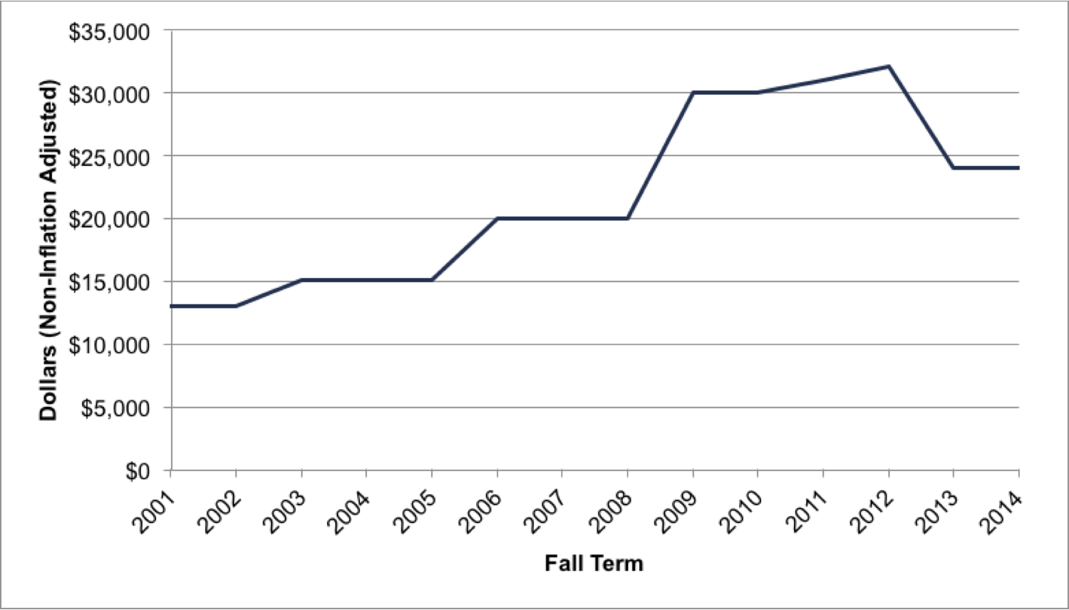
In applying this strategy, we formulate a treatment group and relevant control groups. Constructing the treatment group is relatively straightforward in this case: we examine (1) the sample of students who did not receive an automatic zero EFC in 2008 (the year preceding the policy change) but would have under the new conditions and (2) the sample of students who received an automatic zero EFC in 2009 (the first year of the policy change) but would not have under the old conditions. In other words, our treatment group consists of students with inflation-unadjusted family incomes between $20,000 and $30,000 in 2008 and 2009 who received a Pell Grant. Constructing the control groups is a bit less straightforward. Ideally, for our control groups, we would choose students who have identical (or very similar) characteristics as those students in our treatment group but who were not exposed to the relevant policy change. As there is no “standard” way to approach this, we decide to construct two separate control groups – one each for students with family incomes up to $5,000 above and below the income ranges of the treatment group in 2008 and 2009. The robustness of these control groups is predicated on the fact that the income thresholds for a zero EFC are strict cutoffs. For example, this would mean that a student who had a family income of $30,001 in 2009 might very much resemble another student who had a family income of $30,000 in 2009 (holding everything else constant), but the former would not have qualified for an automatic zero EFC whereas the latter would.^[73] While the higher-income control group appears to serve as a stronger comparison group (as it never qualified for the conditions necessary for an automatic zero EFC in either year), it is nonetheless useful to compare both control groups against the treatment group.

Sample means are provided separately in Table 6.1 for the treatment group and both of the control groups for the year immediately preceding the policy change (2008) and the first year of the policy change (2009). Note that the year-to-year differences in nearly all of the variables uncorrelated with the policy change remain fairly consistent for each group. For example, family incomes declined by an average of less than $100 and SAT scores rose by an average of 15-30 points for each group between 2008 and 2009. For almost all of the other demographic and academic characteristics, the differences between years for each group are all small. However, note that the average EFC values fell by 55% for the treatment group between 2008 and 2009, compared to much smaller decreases of 13% and 4% for the high- and low-income control groups (respectively).^[74] As a result, it is not surprising that students in the treatment group saw significantly larger increases in their grant aid (both Pell and non-Pell) compared to students in both control groups, leading – in turn – to a larger decrease in net cost. Furthermore, we observe that the first-year retention rate increased slightly from 2008 to 2009 for the treatment group, whereas the rate declined or stayed flat for the control groups. Table 6.1 thus provides suggestive evidence that the additivity assumption of the policy change (key to a difference-in-differences estimation strategy) largely holds in this scenario.

Table 6.1. Treatment and Control Group Summary Statistics^[75]

	Treatment Group $20,000-$30,000		Control Group $30,000-$35,000		Control Group $15,000-$20,000
	2008	2009	2008	2009	2008	2009
Family Income ($)	27,368	27,341	35,407	35,344	19,103	19,039
	(3,251)	(3,129)	(1,532)	(1,557)	(1,582)	(1532)
Net Cost ($)	9,405	9,085	9,870	9,962	9,382	9,146
	(4,093)	(4,013)	(4,380)	(4,251)	(4,405)	(4,191)
Budget ($)	20,618	21,769	20,986	21,740	20,636	21,824
	(2,830)	(3,152)	(2,726)	(2,982)	(2,941)	(3,083)
Non-Pell Gift ($)	6,434	7,060	6,888	6,741	6,283	6,980
	(3,830)	(4,007)	(4,303)	(3,970)	(3,693)	(4,285)
Pell Grant ($)	4,797	5,633	4,263	5,038	4,974	5,612
	(701)	(625)	(902)	(1,020)	(695)	(795)
EFC ($)	341	153	879	768	177	171
	(688)	(569)	(902)	(1025)	(702)	(728)
Family Size	3.48	3.47	3.42	3.6	3.19	3.32
	(1.31)	(1.34)	(1.25)	(1.41)	(1.44)	(1.36)
Siblings in College	1.23	1.26	1.24	1.28	1.24	1.28
	(0.47)	(0.51)	(0.5)	(0.56)	(0.53)	(0.56)
SAT (M+V)	995	1023	1015	1035	994	1010
	(174)	(167)	(176)	(161)	(160)	(165)
Black	0.48	0.41	0.46	0.37	0.47	0.45
	(0.50)	(0.49)	(0.5)	(0.48)	(0.50)	(0.50)
Hispanic	0.05	0.06	0.04	0.05	0.05	0.05
	(0.22)	(0.23)	(0.21)	(0.22)	(0.22)	(0.22)
Female	0.62	0.64	0.59	0.6	0.61	0.59
	(0.49)	(0.48)	(0.49)	(0.49)	(0.49)	(0.49)
Age at Entry	18.25	18.26	18.26	18.17	18.30	18.30
	(1.32)	(1.16)	(1.68)	(0.78)	(0.86)	(0.98)
Recent HS Grad	0.91	0.89	0.94	0.87	0.90	0.84
	(0.29)	(0.31)	(0.23)	(0.33)	(0.30)	(0.37)
Campus Housing	0.59	0.62	0.62	0.62	0.56	0.64
	(0.49)	(0.49)	(0.49)	(0.49)	(0.50)	(0.48)
Year 1 Retention	0.85	0.87	0.89	0.83	0.86	0.86
	(0.36)	(0.34)	(0.32)	(0.37)	(0.34)	(0.35)
Year 1 Credits Att.	29.25	29.18	29.22	29.2	29.42	29.02
	(3.10)	(3.09)	(3.12)	(3.04)	(3.43)	(2.93)
Year 1 Credits Earned	0.82	0.87	0.83	0.87	0.80	0.86
	(0.24)	(0.19)	(0.22)	(0.2)	(0.24)	(0.22)
Observations	702	930	449	439	262	365

Results

To robustly demonstrate that the EFC threshold policy change had a statistically significant effect on first-year retention, Table 6.2 reports the results of difference-in-differences regression analyses. In this estimation strategy, the dependent variable is the probability of first-year retention (Year 1 Retention), which is regressed on (1) a binary variable (Post-2009) set to 1 if a student entered an institution in 2009, (2) a binary variable (Treatment) set to 1 if a student had a family income (unadjusted for inflation) between $20,000 and $30,000 (signaling the intention to treat rather than the receipt of the treatment), and (3) an interaction term (Post x Treatment) between the aforementioned binary variables. The reduced form effect of the policy change is captured by the coefficient on the interaction term, controlling for changes over time in average first-year retention rates and average differences in retention for students with incomes between $20,000 and $30,000 and those with incomes immediately above and below this range. As a result, these regressions (and in particular the coefficient on the interaction term) test the hypothesis that any relative changes in the first-year retention rate of students with family incomes between $20,000 and $30,000 can be attributed to the policy change increasing the income threshold required for an automatic zero EFC.^[76]

In Table 6.2, Columns (1) – (3) display the regression results for the higher-income control group and Columns (4) – (6) display the results for the lower-income control group. Focusing first on the higher-income control group (which also provides the stronger comparison), Column (1) presents the most basic regression without any independent variables other than the main binary variables and the interaction term. Column (2) introduces institution fixed effects, and Column (3) adds to Column (2) by inserting a series of student-level covariates. As one can observe, the estimated effect of the policy change on first-year retention changes only slightly with the addition of institution fixed effects and covariates (the vast majority of which are statistically insignificant). This affirms the relatively controlled nature of the initial quasi-experiment. While the standard error (clustered by institution) of the coefficient on the interaction term increases as we add more variables, the policy change in Column (3) still has a positive and statistically significant effect of 5.9 percentage points on the first-year retention rate of students in the treatment group. Furthermore, the explanatory power of the regression rises, as demonstrated by the R-squared increasing from 0.003 in Column (1) to 0.048 in Column (3). While the effect of the policy change using the lower-income control group is no longer statistically significant, the effects are still positive and of a similar magnitude across various specifications in Columns (4) – (6). The lack of statistical significance is not surprising given that the control group was assumed to be less robust in these regressions (since its students automatically qualified for a zero EFC to begin with), but the consistency in both sign and magnitude provides further evidence for the strength of the quasi-experimental strategy.

Table 6.3 displays the results of analyses that test the robustness of our original results to various specifications of the control groups and year ranges (holding everything else constant). The coefficients and standard errors in Table 6.3 correspond to the interaction term Post x Treatment under the full fixed-effects regression previously run in Columns (3) and (6) in Table 6.2. In reshaping first the higher-income control group (initially defined as having inflation-unadjusted incomes of $30,000-$35,000), we created groups with income ranges extending from $1,000 to $10,000. While we find that the effects are smaller and statistically insignificant for the income groups with smallest ranges, the effects for almost all of the other higher-income control groups are between 3 and 6 percentage points and, in several cases, statistically significant at the 90% confidence level.^[77] Modifying the lower-income control group in a similar way, we also find that the effects of the policy across the various ranges – with the exception of the smallest income range – largely resemble the positive and statistically insignificant effect for the original specification.

We also extended the range of our analyses from 2007-08 (examining one year on each side of the policy change) to 2006-10 (two years on each side of the policy change) and find that the effect of the policy for the higher-income control group – while decreasing from 5.9 to 3.5 percentage points – still remains statistically significant at the 90% confidence level. In contrast, the effect of the policy for the lower-income control group fell from 2.7 to 0.6 percentage points while continuing to be statistically insignificant. Finally, we pooled both of our control groups, creating groups with income ranges of $2,500 on each side of the treatment group – corresponding to $17,500-$19,999 and $30,001-$32,500 – as well as $5,000 on each side. The effects are statistically insignificant but of similar magnitude for both manipulations, although the coefficient on the interaction term for the larger pooled sample is only marginally insignificant at the 90% confidence level.

Table 6.2. Difference-in-Differences OLS Regressions

	Higher-Income Control Group			Lower-Income Control Group
	(1)	(2)	(3)	(4)	(5)	(6)
VARIABLES	Year 1 Retention	Year 1 Retention	Year 1 Retention	Year 1 Retention	Year 1 Retention	Year 1 Retention
Post-2009	-0.0557*	-0.0599***	-0.0436*	-0.00790	-0.0165	0.00345
	(0.0303)	(0.0187)	(0.0255)	(0.0344)	(0.0216)	(0.0322)
Treatment	-0.0332*	-0.0278	-0.0233	-0.0107	-0.0146	-0.0313
	(0.0193)	(0.0185)	(0.0266)	(0.0249)	(0.0272)	(0.0409)
Post x Treatment	0.0713***	0.0682***	0.0591*	0.0235	0.0247	0.0269
	(0.0252)	(0.0243)	(0.0292)	(0.0299)	(0.0318)	(0.0376)
Income			1.07e-06			4.43e-07
			(1.85e-06)			(2.59e-06)
Student Budget			-4.97e-06			-5.99e-06
			(4.83e-06)			(6.09e-06)
Family Size			-0.0104			-0.0122
			(0.00775)			(0.00748)
Siblings in College			0.00140			0.0172
			(0.0148)			(0.0194)
SAT (M+V)			6.22e-05			7.31e-05
			(5.99e-05)			(5.88e-05)
Black			-0.00679			0.0129
			(0.0242)			(0.0231)
Hispanic			0.0305			0.0463**
			(0.0210)			(0.0217)
Female			0.0248*			0.0182*
			(0.0135)			(0.0103)
Age			-0.00658			-0.00939
			(0.0113)			(0.0184)
HS Grad. at Entry			0.0594			0.0144
			(0.0370)			(0.0309)
On-Campus House			0.0595*			0.0750*
			(0.0323)			(0.0373)
Local Unemp. Rate			-0.00209			-0.00743*
			(0.00382)			(0.00374)
Constant	0.887***	0.887***	0.943***	0.865***	0.872***	1.064***
	(0.0204)	(0.0114)	(0.236)	(0.0262)	(0.0187)	(0.361)
Observations	2,625	2,625	2,162	2,335	2,335	1,956
Institution FE	N	Y	Y	N	Y	Y
R-squared	0.003	0.038	0.048	0.000	0.038	0.050
Clustered standard errors in parentheses *** p<0.01, ** p<0.05, * p<0.1

Table 6.3. Robustness Checks

		Coefficient	StandardError	Observations	R2
Modifying Higher-Income Control Group	$30,001-$31,000	-0.00601	0.0627	1,570	0.056
	$30,001-$32,000	0.0234	0.0376	1,723	0.050
	$30,001-$33,000	0.0307	0.0370	1,878	0.051
	$30,001-$34,000	0.0513*	0.0300	2,030	0.049
	$30,001-$35,000	0.0591*	0.0292	2,162	0.048
	$30,001-$36,000	0.0617**	0.0276	2,326	0.050
	$30,001-$37,000	0.0551*	0.0271	2,491	0.051
	$30,001-$38,000	0.0407	0.0257	2,636	0.051
	$30,001-$39,000	0.0336	0.0241	2,802	0.049
	$30,001-$40,000	0.0355	0.0267	2,981	0.046
Modifying Lower-Income Control Group	$19,000-$19,999	-0.0486	0.0621	1,527	0.058
	$18,000-$19,999	0.0476	0.0507	1,637	0.063
	$17,000-$19,999	0.0344	0.0391	1,750	0.059
	$16,000-$19,999	0.0260	0.0396	1,860	0.053
	$15,000-$19,999	0.0269	0.0376	1,956	0.050
	$14,000-$19,999	0.0294	0.0321	2,036	0.048
	$13,000-$19,999	0.0181	0.0301	2,118	0.048
	$12,000-$19,999	0.0386	0.0280	2,197	0.047
	$11,000-$19,999	0.0315	0.0258	2,279	0.043
	$10,000-$19,999	0.0284	0.0264	2,338	0.042
Changing Range to ±2 years (2007-10)	Higher-Income	0.0354*	0.0192	4,537	0.042
	Lower-Income	0.00601	0.0218	4,026	0.043
Pooling Samples for Control Groups	±$2,500	0.0321	0.0340	2,075	0.053
	±$5,000	0.0450	0.0287	2,699	0.046
Clustered standard errors are in parentheses *** p<0.01, ** p<0.05, * p<0.1

Consequently, Table 6.3 indicates that the original results found are relatively robust to various categorizations of the control group and time interval examined, thereby giving an additional level of confidence in the difference-in-differences research design.

In summary, we find significant evidence that increasing the income threshold required for an automatic zero EFC – and the implications that such a policy change has for increasing financial aid and reducing net costs – has a strong positive effect on first-year retention. In this particular policy, the change in the income threshold was associated with an average decrease in net costs of nearly $400 for students in the treatment group, which then saw an increase of 5.9 percentage points in the probability of first-year retention. These results, and in particular the causal relationship identified, further provide compelling evidence that there is a statistically significant, inverse relationship between net costs and student retention rates for the lowest income students. Moreover, these new results suggest that the true effect of changes in net costs on student success for poorer students may very well be considerably larger than what we found using the OLS methodology.

Section 7: Reflections on the Future

At a time when the value of higher education is greater than ever before, and policymakers nationwide are calling for increases in college enrollment and degree completion (especially for lower- and middle-income students), public institutions and states must align their financial strategies with efforts to meet these goals.^[78] The evidence in this study strongly suggests that, in states like Virginia, the current funding approach of replacing state appropriations with tuition revenues will have just the opposite effect, leading to lower success rates among all students and widening gaps between students from different socioeconomic backgrounds. In particular, this study demonstrates that this kind of funding shift has the greatest adverse impact on the poorest students, who not only have substantially lower retention and completion rates than their higher-income peers, but also have seen the largest growth in net costs in recent years. As a result, shifting the burden of rising costs from the state to students without significant increases in need-based financial aid will severely limit gains in overall educational attainment, as well as exacerbate already troubling gaps between students from different socioeconomic groups.

Taking advantage of an extraordinarily rich, student-level database assembled over many years, this study documents these findings for the state of Virginia in a way that no previous study has been able to do. However, Virginia and its public institutions are not alone in the challenges that they face. Almost every state saw declines in state funding for public higher education since 2008, accompanied by significant increases in tuition and other student charges. Based on the results obtained in this study, it seems clear that these trends, if continued, will inexorably lead to lower retention and persistence rates for students across the nation, particularly among the poor and near-poor.^[79] Indeed, continuing on this path puts the nation at serious risk of going in exactly the opposite direction of goals set forth by policymakers at all levels to increase student outcomes and close the opportunity gap in higher education.

What can be done to turn the situation around? While there are no simple and quick answers, the national conversation that has been taking place over the last few years offers some possible approaches. In particular, a combination of the following strategies could make a significant impact in Virginia and other states with similar circumstances:

Increasing public funding while also developing an effective performance-based strategy for the distribution of that funding.

As the economy has slowly recovered from the Great Recession, some states have provided modest increases in their funding of public higher education.^[80] Moreover, at least some of these increases have been tied explicitly to improvements in student retention and graduation rates.^[81] While it is still too early to tell how successful any of these efforts will be, we do have some thoughts about how best to proceed in this very complicated area. First, we strongly recommend that such performance-based approaches to the distribution of state funding be accompanied by increases in the overall funding level. Improving student success rates will require investments by the institutions – for increased need-based financial aid, for example – that will be very hard to make when budgets are being reduced or held level.^[82] Second, to be truly effective given the challenges outlined in this report, a performance-based approach to allocating state funds must provide the right kinds of incentives for institutions to improve success rates among those students who are currently the most disadvantaged. While it may be more costly to increase retention and graduation rates at institutions that serve large numbers of poor and near-poor students, these places are where the shortfalls are largest and where the greatest improvements must take place. To make significant progress toward the overall goals, institutions must be provided sufficient incentives – and support – for taking on the challenges associated with these students.

Making enrollment in community colleges more attractive makes sense as a valuable strategic investment only if it moves students closer to the ultimate goals of timely completion of an associate’s degree and a ready, affordable pathway to further education.

Another approach that has received wide discussion is increasing state funding for community colleges to make them more affordable.^[83] This kind of strategy would ideally increase the number of students who ultimately earn an associate’s or bachelor’s degree, and it is appealing in part because of the heavy concentration of low-income students among community colleges enrollees. There is an important caveat, however – the success rates of first-time students enrolling in most community colleges are so low that investing more funds without significantly improving performance at those institutions would have a limited impact on educational levels overall. It might even have a negative effect if it encouraged larger numbers of low-income students to attend community colleges rather than four-year institutions where their retention rates are higher. Making enrollment in community colleges more attractive makes sense as a valuable strategic investment only if it moves students closer to the ultimate goals of timely completion of an associate’s degree and a ready, affordable pathway to further education.^[84]

We recognize that political leaders in many states will be unable or unwilling to increase the level of resources provided to public higher education (no matter how compelling the arguments might seem). Wherever that is the case, we recommend that institutions still proceed aggressively with the kinds of changes described in the following two recommendations. Success in those efforts can produce positive results in terms of the goals and trends laid out in this report, and provide additional evidence to state leaders of the value of deploying additional investments by the state’s public institutions in a targeted way.

Committing to greater efficiency on the part of public systems and institutions.

Public institutions must re-engineer their systems and processes to become significantly more efficient. Even if state funding is increased going forward, it will still be difficult for public institutions in most states to reduce current tuition levels and/or substantially increase financial aid programs based on state funding alone. Indeed, under almost any realistic scenario about state funding, the growing pressure to increase faculty and staff salaries and other ongoing expenses will almost certainly lead to further pressures on tuition.^[85] The institutions themselves must therefore do their part to keep net costs from rising at the same rates in the future, which means that they have to find ways to reduce their own underlying costs. Reducing business-related overhead and instituting more efficient administrative systems and processes are critical elements of such an effort. However, they are not likely to be enough to produce the overall efficiency that is needed to truly “bend the cost curve.” In addition to reducing administrative costs, there needs to be a significant rethinking of the basic processes of teaching and learning.

Technology-based tools are emerging that offer great promise and have the potential to allow a high degree of individualized instruction that can combine with targeted teacher-student interaction to produce instruction that is both effective and efficient.^[86] In addition, the possibility of using data analytics to guide student feedback has the potential to greatly improve student success at a very low cost once the initial investments are made.^[87] More generally, the strategic implementation of these new models of teaching and learning can allow institutions to collaborate much more extensively and achieve significant economies of scale. Increasing enrollment and retention based on upfront investments in technology, with little or no increase in operating costs, would be a big step forward in terms of both greater efficiency and improved success rates.^[88]

Allocating a significant portion of any increased public funding and savings achieved through greater efficiency to need-based financial aid.

Unfortunately, need-based financial aid has not been given a sufficiently high priority in recent years by most states and public institutions. This study demonstrates clearly that the students who are most affected by increasing costs are those from low- and middle-income families, most of whom could not attend any of these institutions without some form of financial aid. Making a clear and substantial commitment to need-based financial aid at both the state and institutional levels would represent a major step forward in making college affordable for this large group of students. Without that kind of commitment, lower-income students will remain much less likely to enroll in a four-year institution and more likely to drop out without earning a degree.

If the overall public goal is to educate and graduate as many students as possible from four-year institutions and reduce the gaps between socioeconomic groups, then both the state and public institutions should be as aggressive as possible about using need-based financial aid to reduce the net costs for students from lower-income families – even if net costs for higher-income students cannot be reduced at the same time. In other words, both state and institutional financial aid programs should be based primarily on need. This principle has generally been accepted for a long time in many states, including Virginia, but recently it has not been funded enough to make college truly affordable for the majority of young people.^[89] If the state is unable to address this issue head-on, increasing overall success rates will continue to be an uphill battle and the gap between lower- and higher-income groups will continue to grow.

Public higher education today is at a crossroads. Rising costs and increasing financial pressures on public colleges and universities across the nation threaten to lower overall educational attainment levels and magnify gaps in income inequality and socioeconomic status. At a time when our economy needs more college-educated workers than ever before, current funding trends in public higher education are leading young people to become less equipped to compete in a 21^st-century world and achieve personal and economic success. We must challenge ourselves – in Virginia and throughout the country – to reverse these trends before they do irreparable damage to the chances of success for entire groups of students and cripple the economies and communities that are dependent on their success. Only then can public higher education in the United States truly fulfill its mission to serve as the greatest engine in our society for economic progress and social mobility.

Appendix

Section A.1: Data and Methodology

State- and Institution-Level Data

State- and institution-level data were used to generate the results reported in Section 3. These data were primarily obtained from SCHEV’s website and the Delta Cost Project Database (IPEDS). A few additional variables were also provided by SCHEV upon request. We aggregated data on undergraduate enrollment, financial aid, tuition charges, and institutional finances. The data received from SCHEV span fiscal years 1993-2015, and the Delta Cost Project data are available for fiscal years 1987-2010.^[90] All monetary values were adjusted for inflation using the “Consumer Price Index for All Urban Consumers: All Items” obtained from the FRED database. CPI values for each fiscal year were created by taking the average of the seasonally adjusted monthly values for September through August.

References to state appropriations correspond to general fund appropriations. We treat non-general appropriations as representative of tuition revenue, and data reported for total revenues and expenditures do not include auxiliary operations. Enrollment data in this section are based on fall headcounts. Calculations of funding per student use the number of in-state FTE students and revenue per student uses the number of FTE students. We chose these definitions to be consistent with the ones used by SCHEV.

Individual Student Data

All results in Sections 3, 4, 5, and 6 are based on individual student-level data collected by SCHEV since the 1997-1998 academic year. These data are reported by each college and university in Virginia, including private institutions and two-year colleges, and go through the spring semester of 2012. They contain information on student characteristics at entry (including SAT score, home zip code, race, gender, high school GPA, etc.), financial information for each year collected from the FAFSA (including family income, expected family contribution, loans offered, total gift and grant aid received, estimated student budget, etc.), student enrollment records, and credit completion. Table A.1.1 describes the variables we used in our study and the number of students for whom we have these data. Each student was tracked for 10 years (20 semesters and 10 summer terms) after entering his/her original institution, and we are also able to link records for students who transferred from one Virginia institution to another.

Table A.1.1. Description of Variables

Variable Name	Description	Median (among in-state students at public institutions)	Number of Observations
Budget (Year 1)	The estimated cost of attendance for a given student, as determined by an institution's financial aid office. This includes tuition and fees, room and board, books, and personal expenses.	$15,306	1,171,492
Total Gift Aid (Year 1)	Amount of gift aid (including grants) a student received in year one	$984	1,027,704
Net Cost (Year 1)	Budget year 1 - Total Gift Aid year 1	$12,664	1,171,492
Total Loans (Year 1)*	Total loans received in year 1	$0	1,027,704
Total Financial Aid (Year 1)*	Total financial aid (loans and gift aid) received in year 1	$4,810	1,027,704
Pell Grant Amount (Year 1)*	Size of the Pell Grant a student received in year one	$0	1,027,704
Pell Grant Flag (Year 1)	An indicator for whether a student received a Pell Grant in year 1	39%	1,027,704
Income (Year 1)*	Individual or Family income (depending on dependent status) from the year prior to entry (as indicated on the FAFSA)	$45,339	756,143
Expected Family Contribution (Year 1)*	Expected family contribution, as determined by the FAFSA based on the family's ability to pay	$3,101	756,143
Need Status (Year 1)	Indicates if a student filed a FAFSA, and whether or not a student received financial aid	74%	1,399,156
Institution	The institution the student attended		1,399,469
Four-year	Whether or institution is a four-year college/university or a two-year college	46%	1,399,469
Public	Whether the institution is public or private		1,399,469
In-state	Whether or not the student was considered in-state when entering the institution		1,399,469
First-time	Whether or not the student was a first-time college student when entering the specified institution	66%	1,399,469
Full-time	Whether the student entered with full-time or part-time status	71%	1,399,469
Reporting Period	The term in which the student entered the institution (fall, spring, summer, fall through spring, or intercession)		1,399,469
Race	Unknown/unreported, African American or Black, American Indian/Native American, Asian and Pacific Islander, Hispanic, White/Caucasian American		1,399,469
Gender	Male, Female or unknown/unreported		1,399,159
Age at Entry	Age of student when s/he entered the institution	19.0	1,250,151
Location of Residence	County in Virginia, or state if out-of-state student		1,399,469
SAT Math and Verbal	Combined math and verbal SAT score	1110	222,216
ACT Composite	Composite ACT score. This was converted to the equivalent SAT score for students without an SAT score	23	28,198
High School GPA	High School GPA (not converted to a uniform scale)	3.49	232,538
Family Size (Year 1)*	Number of family members	3.0	756,129
Family Members in College (Year 1)*	Number of family members in college	1.0	756,135
Dependent Status (Year 1)*	Student is dependent or independent	69%	756,133
Housing Status (Year 1)*	Institutionally Sponsored Housing, non-institutionally sponsored housing, not institutionally sponsored housing or parents' home, parents’ home		1,399,459
Enrollment Status (Semester 1)	All students listed as enrolled		1,399,469
Enrollment status (Semester 2)	Enrolled, dropped out, intermittent enrollment, enrolled at transfer institution, transferred and earned a certificate, transferred and earned an associate’s degree, transferred and earned a bachelor's degree, enrolled and earned associate’s degree, enrolled and earned a certificate, enrolled and earned a bachelor's degree, earned a certificate in earlier semester at original institution, earned an associate’s degree at original institution in earlier semester, earned a bachelor's degree at original institution in earlier semester		1,399,469
Credits Attempted (Year 1)	Number of credits attempted in semesters one and two	24.0	1,238,757
Credits Earned (Year 1)	Number of credits earned in semesters one and two	17.0	1,113,791
Credits Attempted (Semester 1)	Number of credits attempted in semester 1	12.0	1,399,469
Credits Attempted (Semester 2)	Number of credits attempted in semester 2	10.0	1,399,469
Credits Earned (Semester 1)	Number of credits earned in semester 1	8.0	1,399,469
Credits Earned (Semester 2)	Number of credits earned in semester 2	6.0	1,399,469
Credits Attempted (Summer 1)	Number of credits attempted in summer year 1	0	1,399,469
Credits Earned (Summer 1)	Number of credits earned in summer year 1	0	1,399,469
Derived Variables
Income Quintile*	Virginia level income quintiles calculated each year and adjusted for inflation	5	756,143
EFC Quartile*	Expected family contributions are divided into four roughly equal size groups based on the distribution of expected family contribution (inflation adjusted) within all instate students in our dataset	2	629,447
First-Year Retention	Whether or not a student enrolls in the original institution in semester 3 (and was enrolled throughout year 1)	62%	1,304,209
First-Year Persistence	Whether or not a student enrolls at any institution in semester 3 (and was enrolled throughout year 1)	68%	1,304,209
Transfer in First Year	Whether or not a student transfers before semester three	6%	1,304,209
Graduate in Four Years	Whether or not a student graduates in four years	20%	1,012,543
Progress towards a Degree in Four Years	The proportion of credits, out of 30, that a student completes in year one. This is based on the notion that a student should earn 30 credits in year one to make appropriate progress towards a degree in four years.	46%	1,399,469
Success at Two-year College	A student starting at a two-year college is counted as successful if he or she transfers to a four-year college or earns an associate’s degree within two years of entering.	8%	648,579
Transfer from a Two-Year to Four-Year College	Whether or not a student who started at a two-year college transfers to a four year college within two years of entering the two-year college.	4%	648,579
* Only available for students who filed a FAFSA. The budget was imputed for students who did not file a FAFSA based on the average budget for their school within each year.
Note: All dollar values have been adjusted for inflation

Sample of Students

We chose to focus our analyses on first-time, full-time students at public four-year institutions. We include results for students at two-year institutions in Section A.4 of the Appendix, as they are not a part of our primary results. We separate them because we believe that these students are affected by changes in net costs in a different way than students at four-year institutions. In particular, a large portion of the budget for two-year students constitutes living expenses, and less than 20% of a student’s budget represents actual tuition.

We focus on full-time students for two reasons. First, 90% of students at four-year institutions are full-time. Second, the amount of financial aid disbursed usually depends on full-time enrollment status, and it remains unclear how our data on student budget are linked to the number of credits that part-time students take. Tuition is more commonly set at one, or a few, levels for full-time students, so we are able to estimate more precisely their net costs and thus the impacts that these have on outcomes. We choose to focus on first-time students because they are the students for whom we have the most complete data, and they represent the traditional path to a degree. Consequently, if net costs are adversely affecting these students (who are the most successful subsample of students), they are likely affecting other students as well.

All results which focus on net costs rely on a more limited subsample – those students for whom we have accurate financial data. We are only certain that financial data are accurate for students who matriculated in a fall semester and enrolled in both the fall and spring semesters of the academic year. This is because student budget is calculated based on estimated tuition and expenses for an entire year, while the financial aid data report what a student actually received. As a result, a student who only enrolled for one semester would have tuition and expenses estimated for an entire year but have received aid for only one semester, thereby incorrectly inflating his/her net costs. Students who entered in the spring or summer semester are eligible for different (and often smaller) types of financial aid, which once again inflates their net costs. Furthermore, it is unclear how the budget is calculated for these students because of varying practices among the schools in our sample.

Finally, we drop a small group of students who have zero family income at entry but positive expected family contribution because we believe this to be a data error. Families with zero income automatically qualify for zero expected family contribution if they file a FAFSA, and an income value of zero (rather than being missing) for families implies that they filed a FAFSA. Thus, this pattern should not appear in the data. Furthermore, these students appear to be mostly concentrated in a few schools in a few years (and represent a large portion of the student body for those schools in those years), which leads us to believe that these patterns are a result of a reporting or coding error.

Table A.1.2. Student Characteristics by Sample

	(Moving to the right, categories are subsets of the previous one)
	In-State	Four-Year Institutions	First-time, Full-time	Post-2004	Regression Sample*
Net Cost at Entry	$13,120	$16,405	$16,626	$18,004	$16,760
Family Income at Entry	$64,324	$89,856	$97,473	$106,643	$109,605
Income Quintile at Entry	3.7	3.9	4.0	4.0	3.6
Expected Family Contribution at Entry	$9,769	$15,722	$17,455	$20,564	$21,250
EFC Quartile	2.4	2.9	3.0	3.1	3.2
Submitted Financial Data	54%	63%	66%	70%	100%
SAT Math & Verbal	1123	1126	1129	1129	1115
Age at Entry	22.1	19.7	18.2	18.2	18.1
Female	57%	56%	56%	55%	58%
Black	21%	16%	16%	15%	19%
Hispanic	5%	3%	3%	4%	4%
Asian	6%	8%	9%	9%	9%
Race Missing	3%	5%	5%	9%	8%
Unemployment Rate	4.5	4.1	4.1	4.7	4.8
Campus Housing	18%	42%	49%	54%	78%
Dependent	71%	88%	98%	98%	98%
Credits Attempted (Semester 1)	9.6	13.7	14.6	14.7	14.7
Credits Earned(Semester 1)	7.9	12.1	13.0	13.3	13.4
Credits Attempted(Year 1)	18.6	27.3	29.1	29.2	30.0
Credits Earned (Year 1)	15.3	24.0	25.8	26.4	27.3
First-Year Persistence	67%	88%	91%	92%	94%
First-Year Retention	63%	83%	85%	86%	89%
Transfer (Year 1)	5%	5%	6%	6%	5%
Progress to 4-year degree	52%	80%	87%	88%	90%
Graduate in 4 years	21%	45%	43%	47%	47%
Graduate in 6 years	33%	66%	68%	72%	73%
Number of Observations	1,190,444	517,464	391,476	206,857	117,273
*The regression sample is limited to students for whom we have financial data (family income, budget and aid), entered in a fall semester, were enrolled for the fall and spring semesters, and entered after 2003.

Comparing Classifications by EFC Quartiles and Income Quintiles

Income quintiles are used to classify students in Sections 3 and 4 (on trends in net costs and student decisions, respectively). In these sections, we prefer to classify students by income quintiles since they are representative of Virginia’s entire population (and not just the population that attends an institution of higher education), and they allow us to see what portion of the population within each income bracket is attending a postsecondary institution. We turn to EFC quartiles later in the report to minimize the influence that anomalies present in the income data may have on the regression results. As there are more potential student-level errors in the income data than in the EFC data, these can bias the standard errors in the regressions and, as a result, compromise the validity of the results and their statistical significance.

Expected family contribution is calculated based on information on a student’s FAFSA application and takes into account family income, family assets and benefits, the number of siblings in college, and family size. Therefore, it is often considered a better indicator of a family’s ability to pay for college than raw income. In this case, we use it because of the volatility in family income between years and some unusually high levels of EFC reported for low-income students. In particular, it appears that some students who are classified as low-income may not really be “poor,” as they are able to pay a substantial portion of the sticker price. While the presence of these students may bias the micro-level regression analyses, they do not significantly change the analyses of trends in net costs and student decisions aggregated across many students.

We divide EFC into four quartiles based on the within-year distribution of EFC in our sample of all students who entered a Virginia institution between 1997 and 2012. One weakness of this classification is that it is dependent on students enrolling in higher education and submitting a FAFSA, which – unlike income quintiles – does not enable us to compare our sample of students to the population more generally. However, by examining the income levels of students within each of these quartiles, we are able to define groups of poor and near-poor students. The 1^st EFC quartile is entirely composed of students with zero expected family contribution; students in the 25^th percentile of this quartile have an income of $3,948, and those in the 75^th percentile have an income of $24,507. Thus, it appears reasonable to classify these students as poor. In the 2^nd EFC quartile, the students in the 25^th percentile have an income of $26,374, and those in the 75^th percentile have an income of $48,920. We choose to describe these students as near-poor. For a more precise description of the income levels in these bands and for the 3^rd and 4^th EFC quartiles, see Table 5.1 in the main report.

To confirm that the complications in the income data do not substantially bias trends aggregated across students, we analyzed the trends in net costs across a few different subgroups and found similar results to those with the income quintiles. First, Figure A.1.1 demonstrates the similarity in net cost patterns between the EFC quartile and income quintile groupings. Additional graphs with the EFC grouping and/or regression results with the income quintiles are available upon request.

Figure A.1.1. Net Costs by EFC and Income Classifications

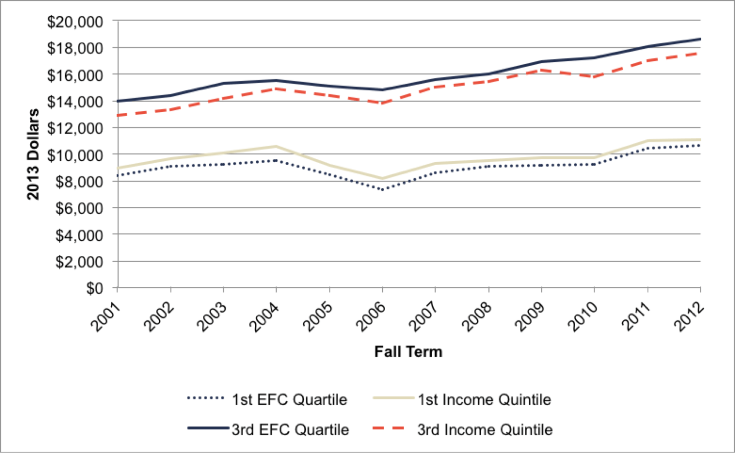
Second, we examined changes in net costs by Pell Grant status, which provides familiar and common definitions of low- and middle-income students. In particular, Figure A.1.2 illustrates how net costs have changed for students who receive Pell Grants, those who receive gift aid but no Pell Grants, and those who receive no gift aid from any source. Much like the patterns associated with income quintiles, net costs prior to 2007 grew most slowly for the “Pell” students relative to the “No Pell with Aid” and “No Aid” students. These patterns reverse once again after 2007, with the average annual growth rate of 4.2% in net costs for the Pell students outpacing the respective 2.7% and 3.2% rates for the “No Pell with Aid” and “No Aid” students during this time period. While we acknowledge that the “No Pell with Aid” and “Pell” student groupings may not be sufficiently concentrated to warrant labeling them as near-poor and poor (respectively), we nevertheless find that the general direction and magnitude of their net cost patterns substantiate the trends associated with students in the lower-to-middle income quintiles.

Figure A.1.2. Changes in Net Costs by Pell Status

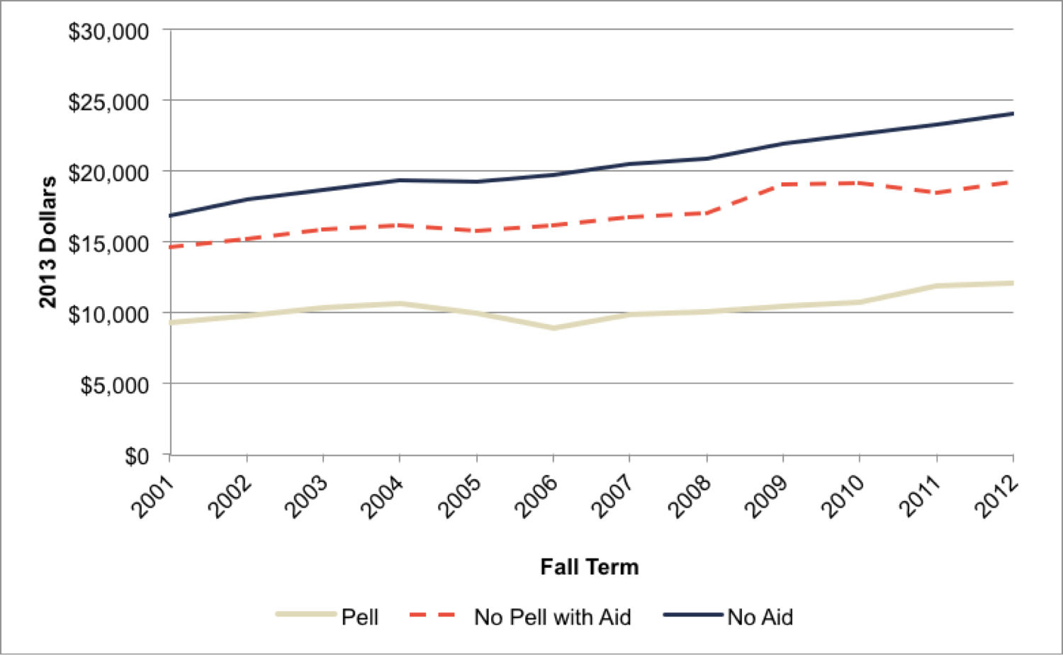
Regression Models

Our three primary regression models are 1) an ordinary least squares (OLS) linear probability model incorporating institutional- and year-fixed effects and standard errors clustered by school and year 2) a discrete-time hazard model estimated using a multinomial logistic regression and 3) a differences-in-differences model.

For the OLS regressions, we focus on results separated by EFC quartile, controlling for various student-level characteristics and institutional- and year-fixed effects. We include control variables for income at entry, expected family contribution at entry, age, race, gender, SAT score, unemployment rate in home zip code, living on campus, and dependent status. In these regressions, we use binary dependent variables for first-year retention, first-year persistence, and four-year graduation (which are each set to 1 if a student is retained, persists, or graduates in four years – respectively – and 0 if not). We also estimate the impact on the number of credits attempted and earned (which each represents a continuous number of credits). Finally, we constructed a progress variable that represents the progress a student makes within year one toward earning a degree in four years (based on the assumption that a student needs 120 credits in four years – and thus 30 credits in each year – to graduate on time). We thus divide the number of credits earned in year one by 30 to create an indicator of progress towards a four-year degree.^[91]

Table A.1.3. Full OLS Regression Results for First-Year Retention

Variables	EFC Q1	EFC Q2	EFC Q3	EFC Q4
Net Cost ($1,000s)	-0.00631***	-0.00472***	-0.00446***	-0.00249***
	(0.00088)	(0.00085)	(0.00061)	(0.00038)
EFC ($1,000s)		0.00061	0.00500***	0.00012**
		(0.00316)	(0.00105)	(0.00005)
Family Income ($1,000s)	0.00003	-0.00003	0.00005	-0.00000
	(0.00023)	(0.00023)	(0.00010)	(0.00002)
SAT (Math + Verbal)	0.00006*	0.00005**	0.00003*	0.00003**
	(0.00003)	(0.00002)	(0.00002)	(0.00001)
Age at Entry	-0.01144**	0.00056	-0.00498	0.00237
	(0.00511)	(0.00504)	(0.00439)	(0.00282)
Female	0.01770***	0.03691***	0.03008***	0.02020***
	(0.00676)	(0.00630)	(0.00438)	(0.00306)
Black	0.01739	0.03717***	0.01727**	0.00507
	(0.01222)	(0.00949)	(0.00711)	(0.00660)
Hispanic	0.02583	0.01131	-0.01762	-0.01617**
	(0.01906)	(0.01289)	(0.01110)	(0.00706)
Asian	0.05318***	0.03844***	0.01255	-0.00216
	(0.01036)	(0.00916)	(0.00835)	(0.00508)
Race unknown	0.01700	0.00344	-0.00399	-0.00958*
	(0.01266)	(0.01152)	(0.00744)	(0.00515)
Unemployment Rate of Home County	-0.00382*	-0.00399*	-0.00253	-0.00135
	(0.00202)	(0.00232)	(0.00166)	(0.00119)
Campus Housing	0.01265	-0.00228	-0.01761**	-0.00436
	(0.01091)	(0.00792)	(0.00701)	(0.00422)
Dependent	0.00874	0.05008	-0.00882	0.10536
	(0.01200)	(0.03190)	(0.03833)	(0.08427)
Year 2005	-0.01311	-0.02304*	-0.01123	-0.00500
	(0.01650)	(0.01369)	(0.00704)	(0.00772)
Year 2006	0.00195	-0.01267	0.01209	0.00472
	(0.01979)	(0.01278)	(0.00865)	(0.00800)
Year 2007	0.01074	0.00714	-0.00031	0.00683
	(0.01776)	(0.01115)	(0.00775)	(0.00560)
Year 2008	0.01324	0.00112	-0.00122	0.00712
	(0.01713)	(0.01215)	(0.00777)	(0.00574)
Year 2009	0.02504	0.01519	0.02483***	0.01802***
	(0.01759)	(0.01168)	(0.00923)	(0.00683)
Year 2010	0.03741**	0.00740	0.02122**	0.02314***
	(0.01847)	(0.01230)	(0.00987)	(0.00757)
Year 2011	0.03105	0.02480**	0.01633*	0.02674***
	(0.02062)	(0.01180)	(0.00926)	(0.00698)
Constant	1.01183***	0.79100***	0.97614***	0.77005***
	(0.10249)	(0.10492)	(0.10800)	(0.09755)
Observations	12,121	13,776	24,636	56,602
R-squared	0.04465	0.03652	0.03537	0.03820
Clustered standard errors are in parentheses. *** p<0.01, ** p<0.05, * p<0.1

A significant advantage of the OLS linear probability model is the ease of interpreting the coefficient on net cost. For the binary dependent variables, the coefficient on net costs represents the change in the probability of being retained, persisting, or graduating in four years (in percentage points) associated with a $1,000 change in net costs. For the continuous variables, the coefficient is interpreted as the change along the scale of the continuous variable – i.e., change in the number of credits earned when net costs change by $1,000.

Institutional- and year-fixed effects enable us to control for differences across institutions and years that may otherwise bias the results when omitted, and we cluster the standard errors by institution and year to account for potential non-independence in observations between these units of analysis. We also estimated a version of our regression that included an institutional-level time trend and found that this did not significantly alter our results.

Section A.2: Robustness Checks

One critique of our OLS models may be that they rely on binary dependent variables in several cases that are usually best suited for continuous dependent variables. While the large size and diversity of our sample reduces the amount of bias usually present when using binary dependent variables within a linear probability model, we tested regressions using probit and logistic models as well to ensure that our original results were not solely a product of the initial specification.

We used a hazard model to compare how net costs influence the likelihood of a particular student outcome compared to other possible student outcomes (e.g., comparing transferring to persisting and remaining enrolled). Here, we include the same set of control variables as in the OLS model, including dummy variables for each year and institution. The hazard model enables us to more effectively compare how net costs push students onto a different path than the binary options (e.g., re-enroll or not) employed in our OLS regressions.

In this model, we view transfer students as separate from those students who persist at the same institution and those who drop out. Transferring may be more desirable than remaining enrolled if students move to a better institution. However, transferring can be a less desirable outcome than remaining enrolled at the same institution if a student cannot transfer all of his/her credits, or the transfer institution is not as good as the original one. Furthermore, transferring can increase time-to-degree and reduce the chances of graduating in four years.^[92]

We run separate regressions for each EFC quartile in order to determine whether net costs have a different type of relationship with student outcomes for different groups of students. We are unable to estimate the multinomial logit regression for the 4^th EFC quartile because we could not find a log-likelihood measure to fit our parameters. We attribute this to the smaller relationship we believe to exist between net costs and student outcomes for higher-income students and the greater variation in EFC that exists in the 4^th EFC quartile compared to the bottom three quartiles. This also fits with the smaller magnitudes we find in the results for the 4^th EFC quartile in the OLS regressions.

Using the same set of control variables and dummy variables for institutions and years, we find that the logistic and probit results exhibit similar patterns to our OLS findings.^[93] As reported in Table A.2.1, the magnitudes are of a similar order across EFC quartiles (although it is difficult to directly compare the magnitude of the coefficients given the different estimation models), and they are in the same direction and have similar levels of significance. Given these similarities, we chose to focus on the OLS results given that their coefficients are easier to interpret and can more easily accommodate institutional- and year-fixed effects.

Table A.2.1. Probit and Logit Results: Impact of a 1% Increase in Net Costs

	First-Year Retention		Four-Year Graduation
	EFC Q1	EFC Q3	EFC Q1	EFC Q3
Logit	0.959***	0.982***	0.952***	0.950***
	(0.00632)	(0.00565)	(0.0124)	(0.00658)
Logit (ln net cost)	0.732***	0.744***	0.745***	0.526***
	(0.0449)	(0.0592)	(0.0566)	(0.0453)
Probit	-0.0232***	-0.00965***	-0.0290***	-0.0312***
	(0.00366)	(0.00304)	(0.00765)	(0.00412)
Probit (ln net cost)	-0.166***	-0.157***	0.0555	0.0696
	(0.0320)	(0.0411)	(0.0397)	(0.0485)
Clustered standard errors are in parentheses and *** p<0.01, ** p<0.05, * p<0.1. All regressions control for income at entry, expected family contribution at entry, age, race, gender, SAT score, unemployment rate in home zip code, living on campus, and dependent status. They also include dummy variables for each year and institution-fixed effects.

To examine whether or not net costs have a linear relationship with student outcomes (as is assumed in the OLS model with the linear net cost variable), we conducted the regression analysis with non-linear forms of net cost. First, we added a quadratic term for net cost to the regression to capture the potential for the effect of net costs to decelerate at higher net cost levels. Doing so did not significantly alter our result, as the relationship between net costs and outcomes was basically linear except at the tails (which we attribute to the outliers). We also estimate the results using the natural log of net costs, which indicates the impact of a 1% change in net cost. As reported in Section 5, we find similar patterns as in the results using the linear form of the net cost variable, although the effects are slightly larger for students with higher net costs (because a 1% increase in net costs for them is larger in magnitude than that for poorer students). These results are reported in Table A.2.2.

Table A.2.2. Results with Alternate Models

		First-Year Retention		Four-Year Graduation
		EFC Q1	EFC Q3	EFC Q1	EFC Q3
OLS No Time Trend		-0.00631***	-0.00446***	-0.00703***	-0.01117***
	($1,000 in Net Costs)	(0.00088)	(0.00061)	(0.00174)	(0.00134)
OLS Time Trend		-0.00647***	-0.00458***	-0.00728***	-0.01118***
	($1,000 in Net Costs)	(0.00089)	(0.00062)	(0.00173)	(0.00135)
Natural Log of Net Cost		-0.03516***	-0.05769***	-0.03516***	-0.12786***
	(1% of Net Costs)	(0.00586)	(0.00768)	(0.00586)	(0.01779)
Net Cost Squared (linear term)		-0.00602**	-0.00862***	-0.01098***	-0.01589***
	($1,000 in Net Costs)	(0.00234)	(0.00159)	(0.00374)	(0.00422)
Squared term		-0.00001	0.00014***	0.00021	0.00017
	($1,000 in Net Costs)	(0.00010)	(0.00005)	(0.00014)	(0.00012)
Clustered standard errors are in parentheses. *** p<0.01, ** p<0.05, * p<0.1. All regressions control for income at entry, expected family contribution at entry, age, race, gender, SAT score, unemployment rate in home zip code, living on campus, and dependent status. They also include dummy variables for each year and institution fixed effects.

Section A.3: Additional Results

Patterns of Student Persistence

In order to better understand student enrollment patterns and how excluding students who are not enrolled over the entire year affects our results, we looked into how many students leave their original institution each semester. We focused on students who entered between 1997 and 2007 in order to follow student patterns for five years.^[94] After four years, 43% of students graduate, 33% leave their original institution, and 24% remain enrolled. The most common time for students to leave is after enrolling for a second semester and before the beginning of the third semester, with 31% of all students who leave within four years leaving at this time.

By limiting our sample to students who are enrolled all year, we lose 35% of the 16% of students who leave during or just after the first year. 6% of all students leave before semester two, and 10% enroll for semester two and leaving during or after it. The rate of students leaving is lower in years two, three and four, but there is still a substantial number of students who do leave during those years.

We focus on persistence and retention between semesters two and three, which is the most common time for students to leave. Our results may underestimate the impacts of net costs if those who leave before the second semester have particularly high net costs (which dissuade them from enrolling for a second term). It is also worth noting that even though four-year graduation rates are low, a substantial number of students remain enrolled after four years and probably earn a degree in five, six or seven years. Unfortunately, we can only perform regression analyses for six-year graduation rates for one cohort of students, and the limited variation in net costs within a single year may bias these results.

Loans

As mentioned in Section 3, many students have coped with increases in net costs by taking out loans. It is thus important to examine if and how these loans impact student outcomes, and if they differ from the role that net costs play in student outcomes. We set up regressions with loans as the primary independent variable, as well as regressions which incorporate both loans and net costs to determine if loans influenced student outcomes beyond their connection to net cost. While the results from these regressions are small, they are generally negative and statistically significant. These results are reported in Table A.3.1.

Table A.3.1. Impact of a $1,000 Increase in Loans on First-Year Retention

	Controlling for Net Costs	Loans as Independent Variable
EFC Q1	0.00233*	-0.00180*
	(0.00124)	(0.00108)
EFC Q2	-0.00053	-0.00255***
	(0.00096)	(0.00093)
EFC Q3	-0.00070*	-0.00156***
	(0.00038)	(0.00037)
EFC Q4	-0.00099***	-0.00120***
	(0.00017)	(0.00017)
Clustered standard errors are in parentheses. *** p<0.01, ** p<0.05, * p<0.1. All regressions control for income at entry, expected family contribution at entry, age, race, gender, SAT score, unemployment rate in home zip code, living on campus, and dependent status. They also include dummy variables for each year and institution fixed effects.

The results in Table A.3.1 indicate that loans have a very small negative influence on first-year retention separate from the effect of net costs. It is only negative and statistically significant at the 99% level for the pooled results and the 4^th EFC quartile. For students in the 1^st EFC quartile, loans actually have a positive result that is statistically significant at the 90% level. By looking at the results with loans as the independent variable, excluding net costs, we see a larger and more statistically significant effect. This suggests that looking only at the relationship between the magnitude of loans and outcomes overestimates how much loans influence outcomes. In reality, a great deal of the relationship between loans and outcomes is related to the large net costs that students with large loans usually face. In fact, it appears that loans – holding other factors constant – may improve outcomes for students in the lowest EFC quartile by providing them a viable means of paying those costs.

As reported in Table A.3.2, loans have a larger and statistically significant negative impact on the number of credits earned in year one. This effect is substantially reduced once we control for net costs, although loans still have an effect above that of net costs. Finally, loans have a significant and negative impact on four-year graduation rates. This effect is largest for the first two EFC quartiles, and is slightly larger than the coefficient on net costs. Consequently, loans appear to have a small negative influence on student outcomes above the impact that net costs have on these outcomes. This is concerning, given that students are simultaneously facing increases in net costs and taking out larger loans. However, the one positive coefficient and the small magnitude of these results indicate that loans are probably not one of the most important influencers of student outcomes.

Table A.3.2. Loans’ Impact on Four-Year Graduation

	Controlling for Net Costs	Loans as Independent Variable
EFC Q1	-0.00645***	-0.00939***
	(0.00244)	(0.00216)
EFC Q2	-0.00644***	-0.00927***
	(0.00177)	(0.00160)
EFC Q3	-0.00315***	-0.00514***
	(0.00076)	(0.00075)
EFC Q4	-0.00338***	-0.00383***
	(0.00040)	(0.00041)
Clustered standard errors are in parentheses. *** p<0.01, ** p<0.05, * p<0.1. All regressions control for income at entry, expected family contribution at entry, age, race, gender, SAT score, unemployment rate in home zip code, living on campus, and dependent status. They also include dummy variables for each year and institution fixed effects.

Section A.4: Funding Trends, Net Costs, and Student Decisions at Two-Year Institutions

Broad financial challenges have also affected public two-year institutions in Virginia, and these developments have, in turn, translated into increased net cost burdens for students at these institutions. We analyze enrollment and outcome patterns among different subgroups of students at two-year institutions before more rigorously examining the relationship between net costs and student outcomes through multivariate regression analyses. While we have chosen to focus our attention in the main report on four-year institutions, we acknowledge the integral nature of Virginia’s two-year institutions within the state’s set of higher education institutions. In particular, we recognize that two-year institutions educate the majority of college-going students in Virginia and that – for some students – they may serve as an important pathway toward a four-year degree. We therefore say a few words here about changes in funding and net costs at two-year institutions, and their impacts on student decisions.

Funding Trends and Student-Level Net Costs

Much like their four-year counterparts, two-year institutions have seen dramatic declines in state appropriations, which fell by 43% between fiscal years 2001 and 2014. With state funding as a share of total institutional revenue dropping from 65% to 45% between 2001 and 2010, two-year institutions have been forced to become increasingly reliant on tuition revenues to balance their budgets. Indeed, in-state tuition charges at two-year institutions increased by a remarkable 120% between 2001 and 2013, compared to a 56% growth in out-of-state tuition charges. Moreover, more than 95% of all students at two-year institutions come from within Virginia, meaning that in-state students have largely borne the brunt of these tuition increases.

As a result, it comes as no surprise that net costs at two-year institutions have increased for students from all income quintiles since the 1997 academic year.^[95] We note, however, that tuition makes up a smaller portion of student budget at two-year institutions than at four-year schools.^[96] Figure A.4.1 (in the same spirit as Figure 3.1 for four-year institutions) demonstrates that net costs since 1997 have risen fastest for students in the highest income quintiles and slowest for those in the lowest income quintile.^[97] Once again, as Table A.4.1 indicates, net costs prior to 2007 grew at an average rate of only 2.0% per year for students in the lowest income quintile (poor), while they actually rose most rapidly during this time period for students in the 3^rd quintile (near-poor). Since 2007, however, net costs grew more substantially for the poor and highest-income students, although we also note that they have dramatically accelerated for poor and near-poor students since 2010. As a result, we observe largely similar patterns over time (albeit with slight variations) in net costs between the public two- and four-year institutions in Virginia, with net costs having increased for all subgroups of students over the past decade but at the most rapid pace in recent years for those students who can least afford a college education.

Figure A.4.1. Changes in Net Costs for Two-Year Institutions

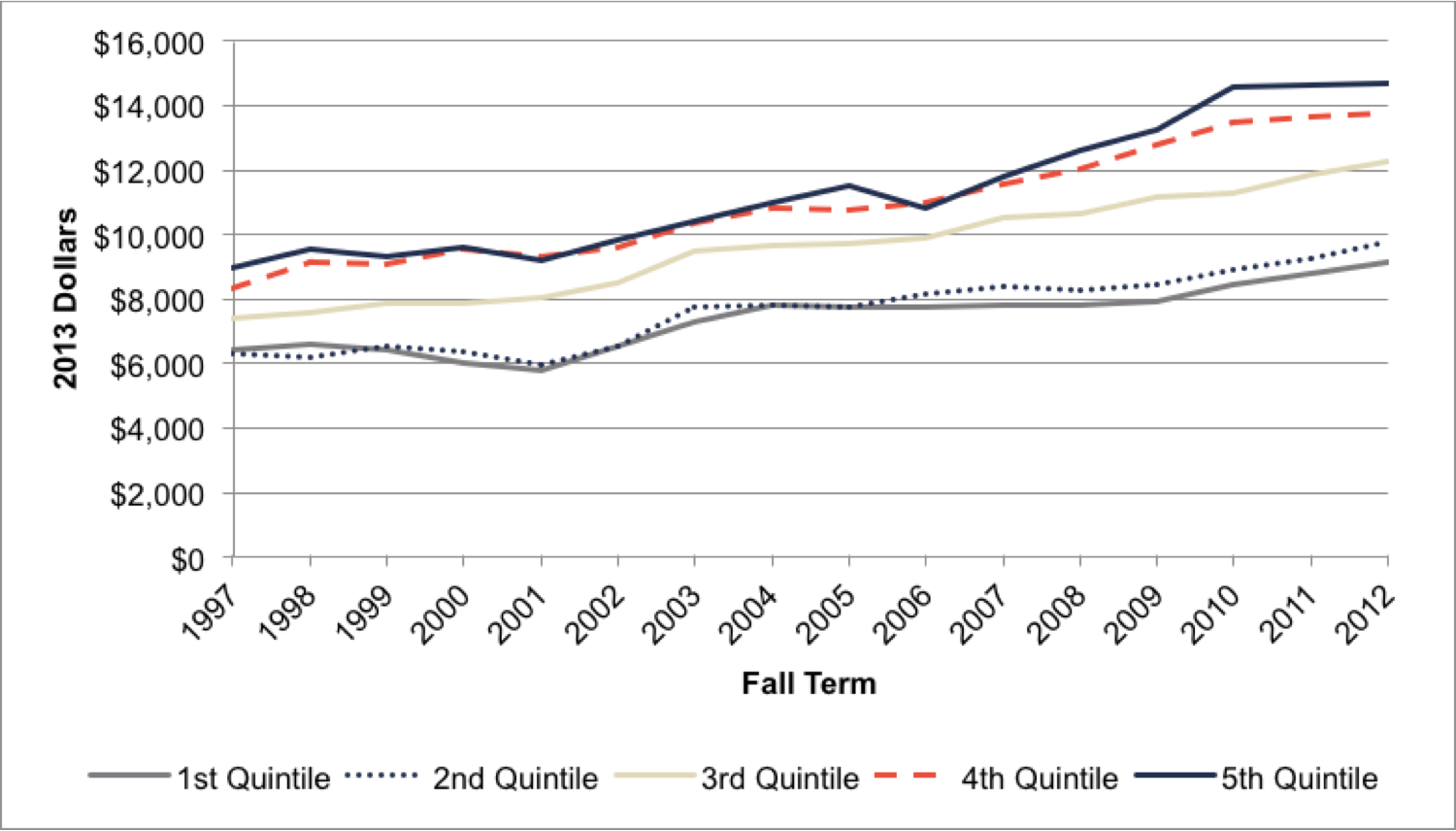
Table A.4.1. Average Annual Growth Rates in Net Costs by Income Quintile

	1st Quintile	3rd Quintile	5th Quintile
1997-2007	2.0%	3.6%	2.8%
2007-2012	3.1%	3.0%	4.4%
Total (1997-2012)	2.4%	3.4%	3.3%

To demonstrate that the recent increases in net costs (especially for lower- to middle-income students) have occurred at nearly every two-year institution, Figures A.4.2 and A.4.3 illustrate institutional-level trends in net costs since 2007 for poor and near-poor students, respectively. As there is a greater disparity in the numbers of students enrolled among the two-year institutions (compared to four-year schools), these figures present individual trends for the four institutions (J. Sargeant Reynolds Community College, Northern Virginia Community College, Thomas Nelson Community College, and Tidewater Community College) that enroll the vast majority of all two-year students, along with the trend for all students attending one of the other twenty two-year institutions. We first notice that the trends for “Other” institutions in both figures track relatively closely – both in direction and magnitude – the net cost patterns averaged across all two-year institutions, which gives us confidence that there do not appear to be any significant outliers among those schools. Furthermore, we observe – particularly in the most recent years – that the patterns in net costs at the four largest institutions have largely reflected the increases in the average trends.

Figure A.4.2. Institutional Net Costs (1^st Quintile)

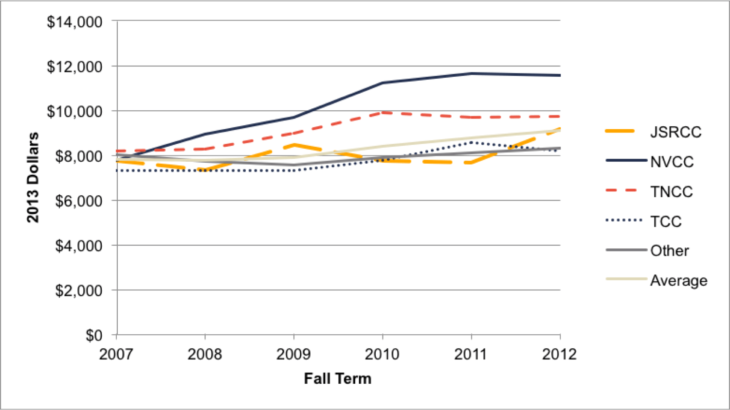
Figure A.4.3. Institutional Net Costs (3^rd Quintile)

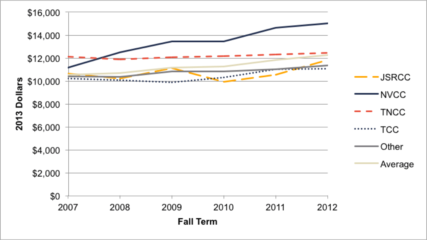
By and large, the recent increases in net costs for students at two-year institutions have been a result of the growth in student budgets outpacing that of gift aid. To demonstrate this, Figure A.4.4 presents the patterns in the components of net costs for students in the 1^st income quintile, who have also experienced the largest increases in net costs in the most recent years. Unlike their counterparts at four-year schools, poor students at two-year institutions receive the majority of their financial aid in the form of Pell Grants (which make up more than 85% of their total award). As we observed with the four-year schools, however, the size of the average Pell Grant award has remained largely constant since 2009, while average student budget levels have increased far more substantially in recent years. Among students in the other income quintiles, we observe similar – albeit more tempered – trends.

Figure A.4.4. Breakdown in Net Costs (1^st Quintile)

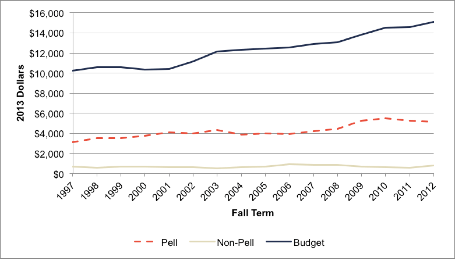
As a result of the increases in student budgets and declines in state appropriations, there have been inflation-adjusted increases in net costs for all student subgroups at two-year institutions. In particular, these trends have accelerated for poor and near-poor students (defined as students with family incomes in the 1^st and 3^rd income quintiles, respectively) in recent years, caused primarily by the inability of financial aid to consistently keep up with rising student charges.

Trends in Student Enrollment and Success

At the same time that net costs have risen for students at two-year institutions, we observe that enrollment has also been rising at an average rate of 6.1% per year for the students in our sample. Figures A.4.5 and A.4.6 break down overall enrollment by income quintiles. While there has been some growth in enrollment among the 2^nd to 5^th income quintiles (particularly since 2006), the largest increases in enrollment have occurred among students in the 1^st income quintile (which, in more recent years, have occurred alongside a substantial decrease in the enrollment of non-FAFSA students).

Figure A.4.5. Trends in Enrollment

Figure A.4.6. Trends in Enrollment Percentage

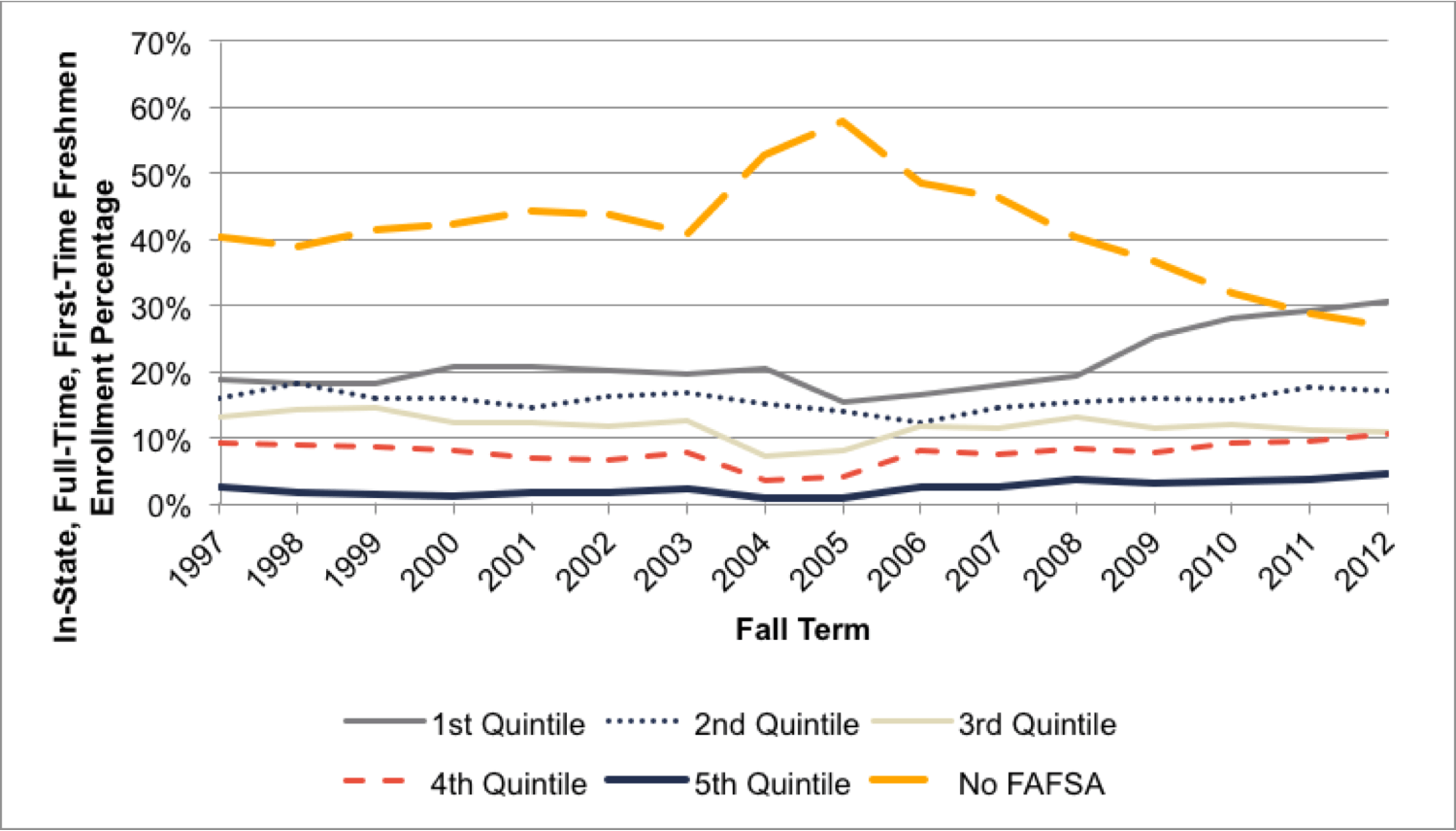
Importantly, the increase in enrollment among poor students was not restricted to only one or a few institutions – as Figure A.4.7 indicates, nearly every two-year institution saw substantial increases in enrollment since 2005. While this increase appears to have tapered off in the most recent years (especially since 2011), it is difficult to conclude based on these figures whether this was a structural change in the underlying trends or merely a year-to-year blip. Nevertheless, Figure A.4.8 demonstrates that the large increase in enrollment among students in the 1^st income quintile may very well have been associated with the growth in the overall population of college-age students across the state. Indeed, the percentage of public, college-enrolling students in Virginia from the 1^st income quintile who started at a two-year institution has held steady at approximately 76%, even as absolute enrollment rose. This troubling statistic contrasts with the comparable percentages for students in the 3^rd and 5^th quintiles, which have held steady at approximately 44% and 11% (respectively) since 2008.

Figure A.4.7. Institutional Trends in Enrollment (1^st Quintile)

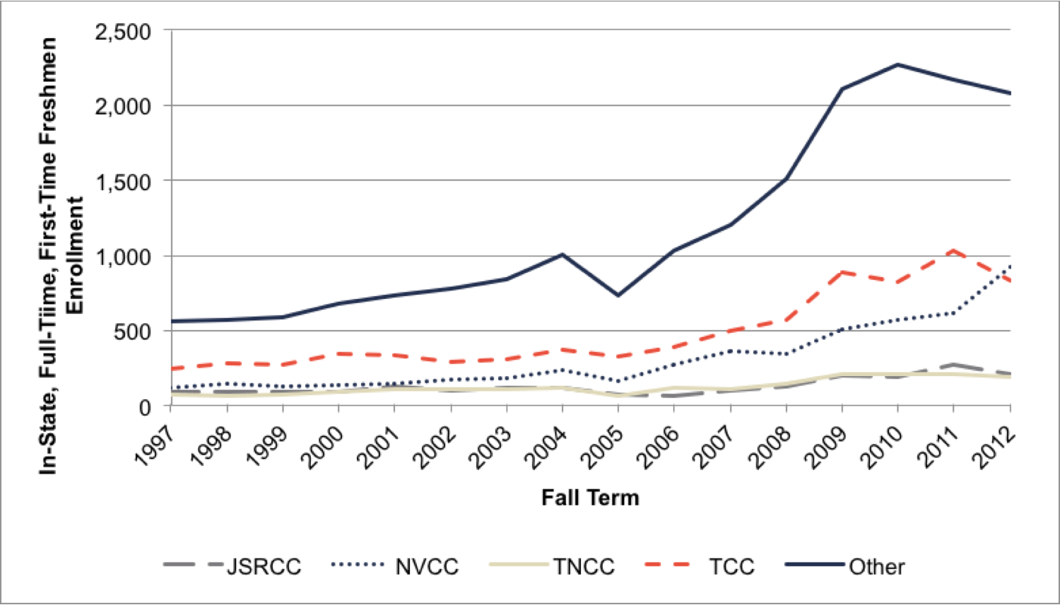
Figure A.4.8. Enrollment as Percentage of Total Statewide Enrollment

Among success measures, we also observe some worrying trends over time – particularly for students in the lower socioeconomic subgroups. Figure A.4.9 disaggregates the first-year retention rate at two-year institutions into patterns by income quintiles. Unsurprisingly, the average first-year retention rate (54%) across all first-time, full-time students at two-year institutions is significantly lower than the comparable rate at four-year schools. From 2010 to 2011, the average retention rate among students in the 1^st income quintile dropped from 52% to 45%, and the gap between the retention rate of the 5^th income quintile students and that of the 1^st income quintile students has been, on average, 15 percentage points. While there are concerns that first-year retention rate might not be as “precise” an outcome measure as first-year persistence rate (given that persistence captures transfer patterns), Figure A.4.10 illustrates that the first-year retention and persistence trends closely track each other over time. As a result, we can conclude that changes in retention rate over time have not been driven by variations in student transfer patterns.

Figure A.4.9. First-Year Retention Rates

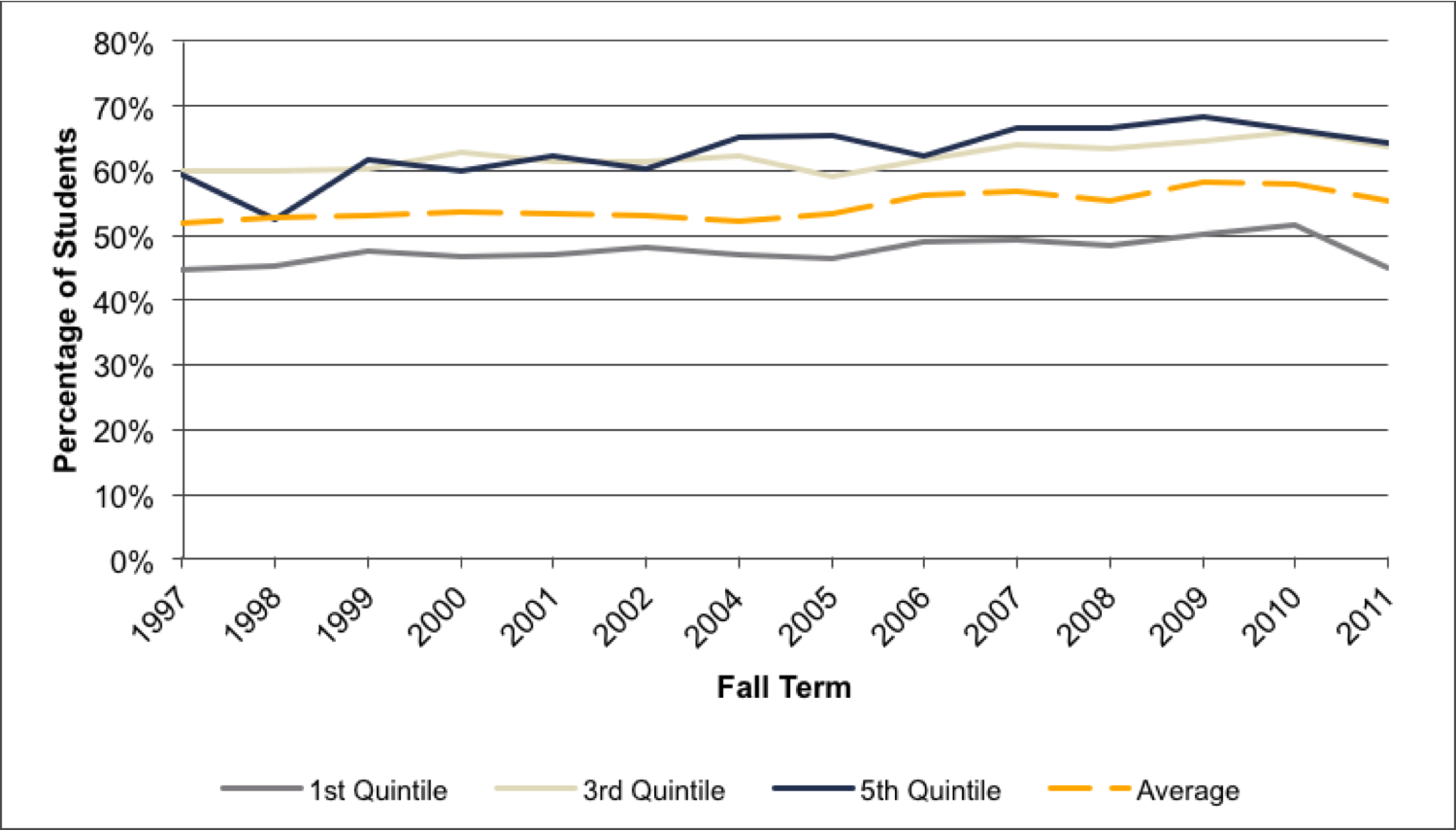
Figure A.4.10. First-Year Retention and Persistence

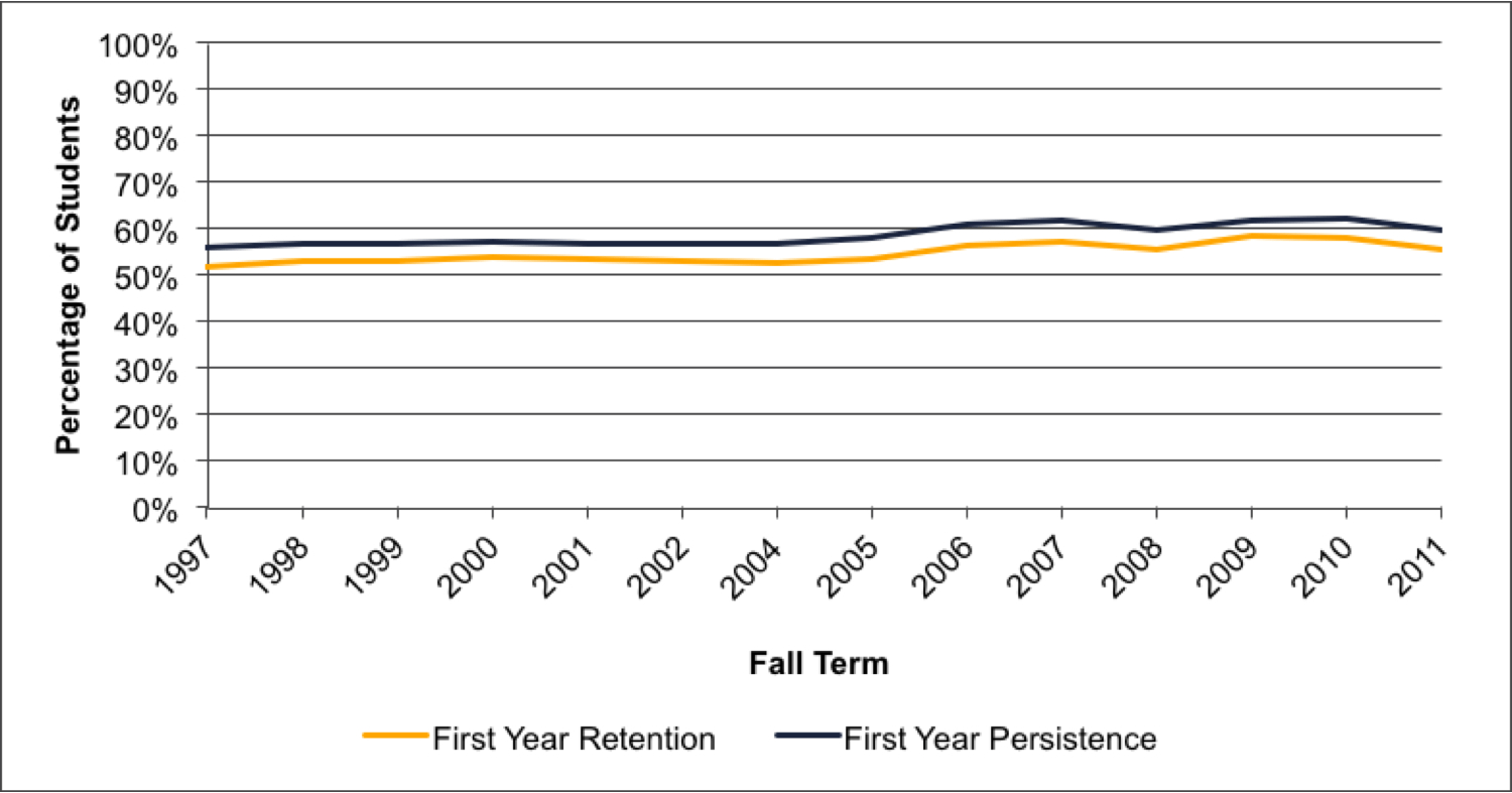
We are also interested in looking beyond students’ first-year outcomes at two-year institutions and assessing how outcomes further into their college careers have changed over time. Figure A.4.11 examines the percentage of students who transferred to a four-year institution within two years of entering a two-year institution. It is apparent from this figure that the oft-discussed pathway of starting and spending two years at a community college before transferring to and finishing at a four-year institution is one that is not well-trodden. Only 5% of all two-year students in our sample actually followed this path, with the rates expectedly below- and above-average for low- and high-income students, respectively. To further broaden our measure of students’ multi-year outcomes, we created a two-year “success variable” that designated whether or not a student either transferred to a four-year institution or earned an associate’s degree within two years of starting at a two-year institution.^[98] Only 8% of all two-year students in our sample are deemed successful according to this measure, with some heterogeneity in magnitudes among low- and high-income students. Furthermore, Figure A.4.12 demonstrates that the trend in this overall success measure has – particularly since 2005 – closely tracked the transfer rate, meaning that changes in the success patterns in recent years were driven not so much by trends in the attainment of an associate’s degree (without subsequently transferring), as they were by changing transfer patterns. These are very discouraging results, especially given that the sample analyzed contains only students who began their time at these colleges on a full-time basis.

Students appear to perform better when given additional time, with the three-year success rate hovering at an average of 17% (Figure A.4.13). While still low, this is markedly better than the two-year success rate.

Figure A.4.11. Percentage of Students Who Transfer to a Four-Year College within Two Years of Entering a Two-Year College

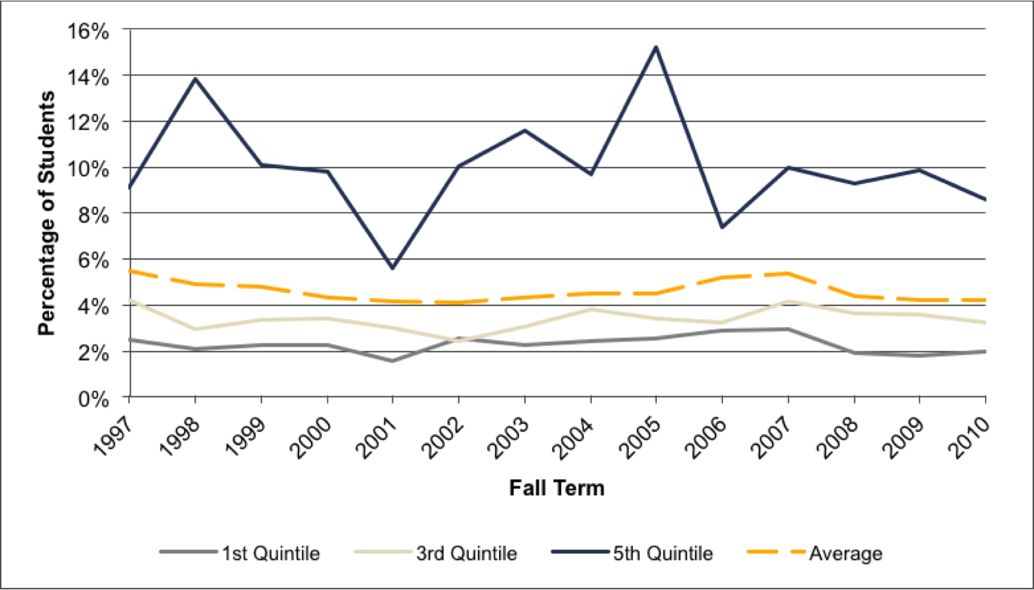
Figure A.4.12. Student Success Rate Compared to Transfer to Four-Year Rate within Two Years

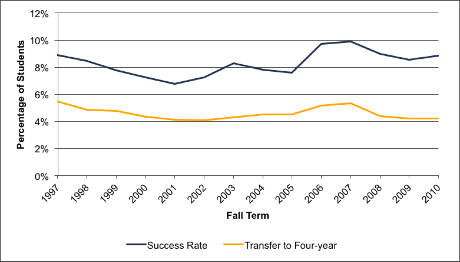
Figure A.4.13. Three-Year Success Rate

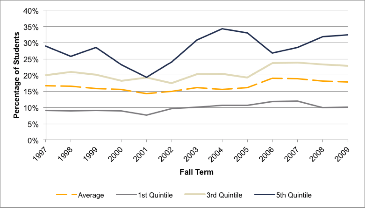
Even among the small fraction of two-year students in our sample who transferred to a four-year institution within two years, only 20% actually graduated within four years of starting at the original two-year institution. While the average rate per year has increased somewhat from 2001 to 2008, this rate still remains worryingly low. As a result, only 2% of all students in our sample actually graduated from a four-year institution within four years of first enrolling full-time at a community college. Six-year graduation rates are slightly better, with 41% of students who transfer to a four-year college within three years of starting at a two-year institution earning a bachelor’s degree in six years (Figure A.4.14). Overall, though, only 5% of students who begin as full-time students at a two-year institution earn a bachelor’s degree in six years.

Figure A.4.14. Average Six-Year Graduation Rate of Two-Year Students (Conditional on Transferring to a Four-Year Institution within Three Years of Starting at Two-Year Institution)

Multivariate Regression Analyses

To assess more rigorously the extent to which changes in student outcomes were associated with changes in net costs, we also ran multivariate regression analyses of various first- and second-year success measures on net cost levels, controlling for a variety of student characteristics as well as institution- and year-fixed effects. While we include all students in our sample from 2001 onwards in our regressions, we are unable to control for specific measures of student academic backgrounds (as the vast majority of two-year students do not have data on SAT/ACT scores and high school GPA). While omitting this variable does not automatically invalidate our results (as academic ability is often correlated with family background measures that are indeed captured in our regression models), it does mean that we should approach these two-year regression results more cautiously than those at the four-year level. Once again, we subdivide students based on their levels of Expected Family Contribution (EFC).^[99]

Table A.4.2 reports the estimated coefficients for the fixed-effects regressions of first-year retention and persistence rates on net costs (in thousands of dollars). An increase in net costs of $1,000 for students in the 1^st EFC quartile is associated with a decrease of 3 percentage points in the probability of retention after the first year and this is statistically significant at the 99% level. This effect decreases in magnitude for students in the higher EFC quartiles. It is important to note that the effects on retention are all statistically significant at the 99% confidence level, and they are above-average (in absolute value) for students in the 1^st, 2^nd, and 3^rd EFC quartiles. These effects contrast with the effect for students in the 4^th EFC quartile, for whom net costs have a small and statistically insignificant effect on retention – signaling that this effect is indistinguishable from zero.

Table A.4.2 also shows that the effects of a $1,000 increase in net costs on the probability of a student at a two-year college persisting after the first year very closely follow the retention effects in direction, magnitude, and statistical significance. While these regressions reflect the functional form of a linear probability model, we have also found that probit and logit regressions show similar results.

Table A.4.3 examines the effects of net costs on other student outcome indicators and finds results strongly corroborating those in Table A.4.1. In particular, an increase in net costs of $1,000 has statistically significant and larger-than-average effects on the number of credits earned and attempted in the first-year, the probability of transferring to a four-year institution, and the two-year success rate for students in the first two EFC quartiles. These results indicate that rising net costs adversely affect student outcomes of various kinds, and those impacts are consistently largest for those students who are least able to afford them.

Table A.4.2. Impact of $1,000 Increase in Net Costs on First-Year Retention

	First-Year Retention		First-Year Persistence
	$1,000 Net Costs	1% increase in Net Costs	$1,000 Net Costs	1% increase in Net Costs
EFC Q1	-0.03033***	-0.15746***	-0.02976***	-0.15873***
	(0.00333)	(0.01817)	(0.00342)	(0.01737)
EFC Q2	-0.02272***	-0.16035***	-0.02366***	-0.16498***
	(0.00284)	(0.01800)	(0.00272)	(0.01697)
EFC Q3	-0.01217***	-0.13353***	-0.00978***	-0.11295***
	(0.00225)	(0.02529)	(0.00205)	(0.02274)
EFC Q4	-0.00431	-0.05793	-0.00297	-0.03342
	(0.00262)	(0.04365)	(0.00231)	(0.04041)
Clustered standard errors are in parentheses. *** p<0.01, ** p<0.05, * p<0.1. All regressions control for income at entry, expected family contribution at entry, age, race, gender, unemployment rate in home zip code, living on campus, and dependent status. They also include dummy variables for each year and institution fixed effects.

Table A.4.3: Impact of $1,000 Increase in Net Costs on Additional Indicators of Student Success at Two-Year Colleges

	Credits Attempted in Year 1	Credits Earned in Year 1	Transfer to a Four Year	Success in Two Years
EFC Q1	-0.38549***	-0.58922***	-0.00233***	-0.00588***
	(0.04250)	(0.07198)	(0.00067)	(0.00136)
EFC Q2	-0.35029***	-0.51742***	-0.00279***	-0.00947***
	(0.05215)	(0.07837)	(0.00092)	(0.00160)
EFC Q3	-0.05603	-0.13059*	0.00197	-0.00226
	(0.05088)	(0.06759)	(0.00124)	(0.00196)
EFC Q4	0.04918	0.05384	0.00178	-0.00113
	(0.06909)	(0.08978)	(0.00160)	(0.00199)
Clustered standard errors are in parentheses. *** p<0.01, ** p<0.05, * p<0.1. All regressions control for income at entry, expected family contribution at entry, age, race, gender, unemployment rate in home zip code, living on campus, and dependent status. They also include dummy variables for each year and institution fixed effects.

1. We would like to thank Peter Blake and Tod Massa for their valuable partnership and engagement in our project.↑
2. We would like to especially thank William G. Bowen, Johanna Brownell, Kevin Guthrie, Martin A. Kurzweil, and Deanna Marcum for their patience and persistence in reviewing multiple versions of this work, and for providing many useful comments, suggestions, and criticisms. ↑
3. While the dataset we received actually contains observations beginning from the 1994-95 academic year, we omit data prior to 1997-98 because of missing financial data for large groups of students in those years. ↑
4. Private colleges and universities generally serve the same broad mission and are an important part of the uniquely American approach to higher education. However, we are focusing in this study on public institutions because it is only the large state-supported public systems that have both the mission and the scale to educate a significant majority of the population.↑
5. President Barack Obama’s “Address to Joint Session of Congress.” February 24, 2009. https://obamawhitehouse.archives.gov/the-press-office/remarks-president-barack-obama-address-joint-session-congress .↑
6. South Korea currently leads the world with 65% of young adult population with college degrees. See “Education at a Glance 2012: OECD Indicators, United States – Country Note.” OECD Publishing (2012). www.oecd.org/unitedstates/CN%20-%20United%20States.pdf .↑
7. See Lumina Foundation’s “Goal 2025” ( http://www.luminafoundation.org/goal_2025 ) and the Bill & Melinda Gates Foundation’s “New Initiative to Double the Number of Low Income Students in the U.S. Who Earn a Postsecondary Degree.” http://www.gatesfoundation.org/Media-Center/Press-Releases/2008/12/New-Initiative-to-Double-the-Number-of-LowIncome-Students-in-the-US-Who-Earn-a-Postsecondary-Degree . ↑
8. President Obama’s “State of the Union Address.” January 20, 2015.http://www.whitehouse.gov/the-press-office/2015/01/20/remarks-president-state-union-address-january-20-2015 . ↑
9. OECD (2012).↑
10. See Table 302.60 from “Digest of Education Statistics.” National Center for Education Statistics (2013). http://nces.ed.gov/programs/digest/current_tables.asp .↑
11. “Institutional Retention and Graduation Rates for Undergraduate Students.” National Center for Education Statistics (May 2014).↑
12. See Figure 2.2 from Bowen, William G., Matthew M. Chingos, and Michael S. McPherson. Crossing the Finish Line: Completing College at America’s Public Universities (Princeton University Press, 2009). Data are derived from NELS longitudinal database, 1988/2000. ↑
13. U.S. Government Accountability Office. “Higher Education: State Funding Trends and Policies on Affordability.” Report to the Chairman, Committee on Health, Education, Labor, and Pensions, United States Senate, p. 1 (2013). http://www.gao.gov/assets/670/667557.pdf .↑
14. Hiltonsmith, Robert & Tamara Draut. “The Great Cost Shift Continues State Higher Education Funding After the Recession.” Demos, p. 2 (2014). http://www.demos.org/publication/great-cost-shift-continues-state-higher-education-funding-after-recession .↑
15. According to the National Bureau of Economic Research, the Great Recession began in December 2007 and ended in June 2009 ( http://www.nber.org/cycles.html ). Thus, throughout the report, we often use 2007 as a turning point.↑
16. Hiltonsmith and Draut (2014), p. 10.↑
17. Hiltonsmith and Draut (2014), p. 12.↑
18. See Figure 2.1 in Section 2 of this report.↑
19. Hiltonsmith and Draut (2014), p. 8. ↑
20. See “State and Country Quick Facts: Virginia,” The United States Census Bureau, December 2014, https://www.census.gov/quickfacts/fact/table/VA/PST045222. Compared to the national average, Virginia has above-average median income, high school completion rates, and bachelor’s degree attainment. If anything, Virginia’s characteristics may underestimate the effect that these financial policies are having in states closer to or below the national average on these measures. ↑
21. In Sections 3 through 6, all years refer to the fall term of an academic year (for example, 2001 represents the 2001-2002 academic year). However, we use fiscal years in Section 2. In Section A.1 of the Appendix, Table A.1.2 describes the sizes and characteristics of different portions of our original population and where they are used in this report. In addition to these students who enrolled in Virginia’s public colleges and universities, our dataset also contains observations for 416,503 students who attended a private institution in Virginia over the same time period. ↑
22. All dollar numbers and growth rates for dollar amounts are adjusted for inflation. ↑
23. See Long, Bridget T. and Michal Kurlaender. “Do Community Colleges provide a Viable Pathway to a Baccalaureate Degree?” Educational Evaluation and Policy Analysis 15, no. 1 (2015): 30-53. Even after controlling for differences in academic preparedness and other student-level characteristics, Long and Kurlaender (2009) find that students who start at community colleges are 14.5% less likely to complete a bachelor’s degree in 9 years than students who started at a four-year institution.↑
24. We are unable to carry out similar regressions to determine the effects of net costs on the likelihood of enrollment, since our data encompass only those students who have already enrolled. ↑
25. Leonhardt, David. “The Great Wage Slowdown, Looming Over Politics.” The New York Times, November 11, 2014. http://www.nytimes.com/2014/11/11/upshot/the-great-wage-slowdown-looming-over-politics.html?_r=0 .↑
26. The exact windows of time vary slightly depending on the dataset that we use. The SCHEV data are available from the 1993 to 2014 fiscal years and the Delta Cost data are available from 1987 to 2010.↑
27. This calculation includes all in-state undergraduate, graduate, and professional students who comprise those students that the state takes into account when determining funding levels. Data are only reported until 2010 for individual two-year institutions. However, all two-year institutions saw a decline in state funding per student between 2001 and 2010. Since average funding for two-year institutions continued to decline through 2012, it is likely that all two-year institutions had lower funding in 2013 than they did in 2001. ↑
28. “2014-2015 Tuition and Fees at Virginia’s State-Supported Colleges and Universities.” State Council of Higher Education for Virginia, https://rga.lis.virginia.gov/Published/2015/RD191/PDF. ↑
29. To put this in perspective, state appropriations per student between 2000 and 2013 declined from $11,344 to $6,160 and $5,240 to $2,967 at four-year and two-year institutions, respectively.↑
30. This represents an increase of 37,269 and 57,463 in-state students at four- and two-year institutions, respectively. As a result, while the dollar amount in state appropriations in 2014 was greater than its comparable level in 1994, average funding per student is now 24% lower. The increases in enrollment across two-year and four-year systems are also similar, and the percentage of total students enrolled at two-year institutions has remained roughly the same since the early 1990s – 52% in 1994 compared to 54% in 2014. Furthermore, the relative amounts of funding directed to the two-year and four-year systems have remained largely unchanged in the face of limited public funds.↑
31. All references to enrollment and enrollment growth in this section use the headcount definition, although the per-student funding trends in Figures 2.1 and 2.2 designate appropriations per FTE enrollment. We employ this distinction to be as consistent as possible with the definitions used by SCHEV. Alternate definitions of enrollment do not substantially alter the results or trends.↑
32. “The Erosion of State Funding for Virginia’s Public Higher Education Institution.” State Council of Higher Education for Virginia, p. 10 (2009), https://files.eric.ed.gov/fulltext/ED511012.pdf. ↑
33. The HDS institutions all relied on state appropriations for at least 35% of their total revenue in 2009-10, ranging from 36% to 52%. The LDS institutions were all below 30% on the same measure, ranging from 10% to 29%.↑
34. This is because in-state tuition charges are lower than average total revenue per student. Thus, as more students enroll, state appropriations per student decline and average total revenue per student declines as well. ↑
35. Net tuition revenue is the amount of money the institution takes in from students after institutional grant aid is provided. ↑
36. This is advantageous since increasing in-state enrollment (while bringing in more total tuition revenue) would otherwise result in a reduction in revenue per student (holding everything else constant), given that the marginal in-state tuition revenue gained from an extra student is less than the average current revenue per student.↑
37. It is also important to note that these financial data for two-year institutions are only available for the system at the aggregate level. It is possible that institution-level data would reveal variations across institutions that might make our interpretation of the situation somewhat different. ↑
38. The recent policy changes at the University of Virginia and the College of William & Mary are excellent examples of the types of decisions institutions will likely have to make. The University of Virginia decided to reduce funding for its financial aid program, AccessUVA, while William & Mary opted to go in the other direction by instituting very large tuition increases that were in part designed to provide significant amounts of additional funding for financial aid.↑
39. We refer to an academic year by its fall term. Thus, the 1997 academic year represents Fall 1997-Spring 1998. Throughout the report, all years refer to the fall term of the academic year.↑
40. For the work reported in this section, we first dropped students who had family incomes of zero but non-zero levels of expected family contribution (EFC). This adjustment is meant to address a few instances in which the vast majority of students at a particular university in a specific year had missing income data that were converted to zero EFC data. Second, we dropped students who left an institution before the end of an academic year. This is due to a discrepancy in the time frame in which the components of net cost are reported, resulting in data that showed abnormal and inaccurate estimates of net costs for those students. A description of the students excluded from our analysis is provided in Section A.1 of the Appendix.↑
41. A student’s budget comprises total estimated cost of attendance, including tuition and mandatory fees, as well as allowances for room and board, books and supplies, childcare, and personal expenses. Tuition and mandatory fees have also increased by almost the same amount as budgets for all students in recent years, suggesting that the trends in net costs that we observe in this section are primarily the result of increasing institutional charges and changes in financial aid, and not by the non-institutional components of a student’s budget. ↑
42. We are grateful to Kirby Posey of the U.S. Census Bureau for providing us with historical data on state-level income quintiles.↑
43. Our sample of interest only includes students who filled out FAFSA forms and thus have family income data. If most students who choose not to fill out FAFSA forms come from the highest income group, our net cost and income numbers for students in the 5^th quintile might slightly understate the true numbers faced by students in that income group. ↑
44. We also find that the trend in average net costs for students in the 5^th quintile behaves similarly to that of their average student budget (which presumably reflects the net costs paid by non-FAFSA students who receive no need-based aid).↑
45. Average annual growth rates are calculated by taking the geometric mean of each year’s annual growth rate. ↑
46. It is important to recognize that net costs for poor and near-poor students were never low to begin with. In 2007 (which proved to be one of the “cheapest” years during this entire time period), poor students paid an average of $9,262 in net costs (in 2013 dollars), with this value rising to $11,010 in 2012. As Table 3.1 indicates, this group of students has a median family income of $14,912, implying that college costs place a very large financial burden on these families even after factoring in need-based financial aid.↑
47. The trend for the 1^st income quintile omits observations from one university in 2007, as there were a nontrivial number of students with family incomes recorded as zero in that year, which is inconsistent with patterns both before and after 2007. ↑
48. Table 3.3 calculates the standard deviation between institutions in the rate of change of net costs rather than in the magnitude of net costs. We are less concerned in this study about institutional differences in net cost levels than we are about institutional differences in how net costs have changed. Due to institutional anomalies in the data, the standard deviation in Table 3.3 omits the data from three different institutions in three different years.↑
49. We found that 2010-11 marked the first instance since 2001 that both the exogenous (federal) and endogenous (state/institutional) sources of financial aid decreased in the same year for poor students. Furthermore, we found that more than 61% of the change in net costs since 2010 can be attributed to the decline in gift aid (with nearly two-thirds of that share ascribed to the decrease in state/institutional aid).↑
50. These values are calculated by multiplying the number of students from the 1^st and 3^rd income quintiles enrolling in four-year institutions between 2007 and 2012 by the average increase in net costs during the same time period for these quintiles. ↑
51. Given the year ranges that we examine, we analyze patterns in first-year retention and four-year graduation between 1997 and 2011 and 1997 and 2008, respectively.↑
52. Although the growth in enrollment for students in our sample has slowed since the beginning of the recession, the enrollment of students outside our sample (i.e., non-first-time, part-time, and out-of-state students, as well as those at two-year institutions) has been growing at a faster rate in recent years. As a result, overall enrollment among all students in Virginia has been rising faster since the Great Recession (as described in Section 3).↑
53. Because of missing family income data for students at one institution in 2006, another institution in 2007, and a third institution in 2012, we impute enrollment estimates for these institutions/years by averaging the numbers for the year preceding and following the year with missing data.↑
54. This effectively allows us to control for broader factors (e.g., state policies, population growth) that might influence enrollment patterns of different groups. More than 87% of all in-state, full-time, first-time freshmen since 1997 in our dataset attended a public institution.↑
55. Thus, the growth in enrollment observed in Figures 4.2 and 4.3 for students in the 1^st income quintile was not a phenomenon isolated only to four-year institutions, as enrollment also grew significantly for the poor at public two-year institutions as well. ↑
56. Thus, out of all first-year students, 6.2% transfer, 4.5% drop out, and 4.7% take time off in their first year. ↑
57. We are unable to conduct these analyses for the initial enrollment decision because we have data for students who actually enrolled but do not have similar information about students who did not enroll anywhere in the system.↑
58. All results done by income quintile are available upon request. In addition, all results in the previous sections reported by income quintile are also available by EFC quartile. The Appendix includes a graph displaying the mean net cost by EFC quartile over time. ↑
59. Definitions of all variables used in the report are provided in Section A.1 of the Appendix.↑
60. More details on the setup and advantages of the hazard model can be found in Section A.1 of the Appendix. ↑
61. The median net cost for the 1^st EFC quartile is $9,055, $11,042 for the 2^nd EFC quartile, $16,456 for the 3^rd EFC quartile, and $20,448 for the 4^th EFC quartile. ↑
62. Progress is a continuous variable calculated as the number of credits completed in year one divided by 30, since 30 is the number needed to be on track for graduating in four years. Progress is a good way of measuring movement towards earning a four-year degree. It is more related to first-year factors and net costs than four-year graduation because there are several factors in subsequent years that can deter or encourage a student to graduate in four years. However, it is clear that completing the recommended number of courses in one’s first year is a big step towards graduating in four years. McCormick and Carroll (1999) find that 91% of students who completed 30 credits in their first year at a four-year institution earned a degree. See McCormick, A. C. and C.D. Carroll. “Credit Production and Progress toward the Bachelor’s Degree: An Analysis of Postsecondary Transcripts for Beginning Students at 4-Year Institutions.” Washington, DC: U.S. Department of Education (1999).↑
63. Results for these additional outcome measures when using the natural log of net costs are reported in Section A.1 of the Appendix. ↑
64. We looked into the impacts of second and third year net costs on outcomes during these years, but anomalies in the data prevented us from being able to derive meaningful results.↑
65. Bettinger, Eric. “How Financial Aid Affects Persistence.” In College Choices: The Economics of Where to Go, When to Go, and How to Pay For It (University of Chicago Press, 2004), p. 207-238.Castleman, Benjamin L. and B.T. Long. “Looking Beyond Enrollment: The Causal Effect of Need-Based Grants on College Access, Persistence, and Graduation.” National Bureau of Economic Research Working Paper 19306 (2013).http://www.nber.org/papers/w19306. Goldrick-Rab, Sara, Douglas N. Harris, Robert Kelchen, and James Benson. “Need-Based Financial Aid and College Persistence: Experimental Evidence from Wisconsin.” Institute for Education Sciences. October 10, 2012. https://papers.ssrn.com/sol3/papers.cfm?abstract_id=1887826.↑
66. This is different from the interpretation of the coefficients from the OLS results. Here, the coefficients represent percent changes – a coefficient of 1.0617 would represent an increase in the likelihood of not being retained by 0.617% of 78% (or approximately 0.48 percentage points) when net costs increase by $1,000.↑
67. We were unable to estimate a log likelihood relationship for the 4th EFC quartile because the maximum likelihood estimation fails to converge for the 4th EFC quartile. This may be due to the small number of students in this group who transfer or do not persist.↑
68. We do not have enough independent students in our sample of first-time, full-time students at a public four-year institution to conduct regression analysis only for them.↑
69. Angrist, Joshua, Daniel Lang, and Philip Oreopoulos. “Incentives and Services for College Achievement: Evidence from a Randomized Trial.” American Economic Journal: Applied Economics 1, no. 1 (2009): 136-163.Dynarski, S. “Building the Stock of College-Educated Labor.” Journal of Human Resources 43, no. 3 (2008): 576-610.↑
70. See 2007 College Cost Reduction and Access Act ( http://www.finaid.org/educators/HR2669_conf_report.pdf ). All of the reported numbers in this section reflect their original year (i.e., unadjusted for inflation), but all of the analyses done with the data are adjusted for inflation.↑
71. See 2009-10 EFC Formula. ↑
72. While there was also a sharp decline in the income threshold from 2012 to 2013 (which would actually correspond more directly with the phenomenon of rising net costs that we have documented), this change occurred outside of the range of our student-level dataset. ↑
73. This is not to say that the student with family income of $30,001 would not have ultimately received a zero EFC, but merely that this student would not have automatically qualified for one.↑
74. The average EFC value for the treatment group in 2009 is not zero (as one would expect after the treatment), since we are only able to isolate those students who qualified for the income cutoff necessary for an automatic zero EFC and not any other necessary conditions. To the extent that having a Pell Grant serves as a proxy for the second condition, we have done our best to isolate the students in the treatment group to those who would have qualified for an automatic zero EFC under the policy change. Indeed, 78% of students in the treatment group in 2009 received a zero EFC (compared to only 55% in 2008). ↑
75. These numbers are all adjusted for inflation (e.g. the $20,000-$30,000 income group refers to, in 2013 dollars, the $21,817-$32,729 group in 2008 and the $21,769-$32,653 group in 2009). Standard deviations are in parentheses. ↑
76. For example, even though there was a concurrent policy change during these years that increased the average Pell Grant for lower-income students, we can be reasonably confident that the effect captured by our regression is “uncontaminated” by such a policy, as the treatment and both control groups were both exposed to such a policy. ↑
77. While it may seem strange that the coefficients are smallest and statistically insignificant for the control groups that most “resemble” the treatment group, this may be attributed to (1) a very small sample size for the control groups and (2) the strict EFC cutoff not being implemented as cleanly in practice. ↑
78. Baum, Sandy. “Higher Education Earnings Premium Value Variation and Trends.” Urban Institute (February 2014). https://www.urban.org/research/publication/higher-education-earnings-premium-value-variation-and-trends. See also Obama (2009), Lumina Foundation’s “Goal 2025,” and the Bill & Melinda Gates Foundation’s “New Initiative to Double the Number of Low Income Students in the U.S. Who Earn a Postsecondary Degree.”↑
79. See Hiltonsmith and Draut (2014), p. 2 and U.S. Government Accountability Office (2014), p. 11. ↑
80. “State Higher Education Finance FY 2013.” State Higher Education Executive Officer, p. 7 (2014). https://sheeo.org/wp-content/uploads/2019/03/SHEF_FY13-2.pdf.↑
81. Fain, Paul. “Scorecard for Scorecards.” Inside Higher Ed. October 29, 2013.https://www.insidehighered.com/news/2013/10/29/complete-college-america-report-tracks-state-approaches-performance-based-funding .↑
82. Some states, including Virginia, have been trying to implement such performance-based approaches even while continuing to reduce state funding. See Virginia Higher Education Opportunity Act of 2011:http://lis.virginia.gov/cgi-bin/legp604.exe?111+ful+CHAP0828+pdf .↑
83. See, for example, the Tennessee Promise: https://www.tn.gov/tnpromise.html and The White House’s proposal for “Tuition-Free Community College for Responsible Students”: http://www.whitehouse.gov/the-press-office/2015/01/09/fact-sheet-white-house-unveils-america-s-college-promise-roposal-tuitio. ↑
84. Brooks, David. “Support our Students.” The New York Times. January 19, 2015. http://nyti.ms/1yjs3wvVara, Vauhini. “Is College the New High School?” The New Yorker. January 13, 2015. http://www.newyorker.com/business/currency/college-new-high-school .↑
85. Flaherty, Colleen. “Professor Pay Up 2.2%.” Inside Higher Ed. April 7, 2014. https://www.insidehighered.com/news/2014/04/07/faculty-salaries-are-22-report-sees-many-financial-issues-facing-professors .↑
86. Bowen, William G., Matthew M. Chingos, Kelly A. Lack and Thomas I. Nygren. “Interactive Learning Online at Public Universities: Evidence from a Six-Campus Randomized Trial.” Journal of Policy Analysis and Management 33, no. 1 (2014): 94-111.Means, Barbara, Yukie Toyama, Robert Murphy, and Marianne Baki. “The Effectiveness of Online and Blended Learning: A Meta-Analysis of the Empirical Literature.” Teachers College Record 115, no. 3 (2013): 1-47.Marcum, Deanna, Christine Mulhern, and Clara Samayoa. “Technology-Enhanced Education at Public Flagship Universities: Opportunities and Challenges.” Ithaka S+R (December 2014).http://www.sr.ithaka.org/research-publications/technology-enhanced-education-public-flagship-universities .↑
87. Dietz-Uhler, Beth and Janet E. Hurn. “Using Learning Analytics to Predict (and Improve) Student Success: A Faculty Perspective.” Journal of Interactive Online Learning 12, no. 1 (2013):17-26. http://www.ncolr.org/jiol/issues/pdf/12.1.2.pdf .↑
88. Deming, David J., Claudia Goldin, Lawrence F. Katz, and Noam Yuchtman. “Can Online Learning Bend the Higher Education Cost Curve?” NBER Working Paper No. 20890 (2015). ↑
89. Sanchez, Claudio. “How the Cost of College Went from Affordable to Sky-High.” National Public Radio. March 2015. http://www.npr.org/2014/03/18/290868013/how-the-cost-of-college-went-from-affordable-to-sky-high . ↑
90. We convert these to academic years in the body of the report for consistency. ↑
91. This variable is not top-coded, so a student could have a progress level greater than one. ↑
92. Cullinane, Jenna. “Transfer and Time to Degree: A Quasi-Experimental Study of Credits, Preparation, and Pace.” In Annual Meeting of The Association for Education Finance and Policy (February 28, 2014). San Antonio, Texas.↑
93. We estimate separate regressions with the linear term of net costs and then with the natural log of net costs. ↑
94. Some of the estimates for graduation and persistence may be 1-2 percentage points different than the numbers reported in the text because we are reporting for slightly different years here. We omit 2008 graduation rates in our averages in this section and persistence rates for 2008-2012 so that we can follow the same sample for five years. ↑
95. Once again, we examine the sample of students encompassing in-state, first-time freshmen attending two-year institutions on a full-time basis (at entry). While we recognize that eliminating part-time students from the two-year institution sample might more significantly skew this sample’s reflection of the overall population than in four-year institutions (given that part-time students make up a much larger subset of the overall student body at two-year schools), we had to restrict our sample in such way because of the manner in which net cost data are compiled. In particular, we see little – if any – evidence that the budget values for students reflect their full-time or part-time status. ↑
96. We are less confident that increases in student budget at two-year institutions have been primarily driven by tuition increases. At the same time, we still note that average tuition rates at two-year institutions have been increasing faster than average levels of gift aid in recent years.↑
97. For the remainder of this section we refer to academic years where the year noted is the fall term. For example, the 1997-1998 academic year is referred to as the 1997 fall term. ↑
98. As a result, the fraction of students who transferred to a four-year institution within two years of starting at a two-year institution (Figure A.4.11) is a proper subset of the set of students who are deemed as “successful.” The difference between the “transfer” and “success” variables lies in the students who graduated with an associate’s degree within two years but did not transfer. ↑
99. For an explanation of why we divide by EFC instead of income quintile, see Appendix Section A.1. ↑